
Abstract
Early fault detection and diagnosis of grid-connected photovoltaic systems (GCPS) is imperative to improve their performance and reliability. Low-cost edge devices have emerged as innovative solutions for real-time monitoring, reducing latency, and improving response times. In this work, a lightweight Convolutional Neural Network (CNN) is designed and fine-tuned using Energy Valley Optimizer (EVO) for fault diagnosis. The CNN input consists of two-dimensional scalograms generated using Continuous Wavelet Transform (CWT). The proposed diagnosis technique demonstrated superior performance compared to benchmark architectures, namely MobileNet, NASNetMobile, and InceptionV3, achieving higher test accuracies and lower losses on binary and multi-fault classification tasks on balanced, unbalanced, and noisy datasets. Further, a quantitative comparison is conducted with similar recent studies. The obtained results indicate good performance and high reliability of the proposed fault diagnosis method.
Introduction
Fossil-based sources are anticipated to maintain their dominance in the energy sector in the forthcoming period, as contended by the Organization for Economic Co-operation and Development (OECD)1. This dominance persists despite global energy consumption experiencing a significant increase, rising from 270.5 exajoules (EJ) in 1978–580 EJ by 2018. Such a notable escalation in energy usage can be attributed to the substantial growth in the global population, which reached 7.63 billion in 2018, marking a 77% increase from 4.30 billion in 19782. Fossil fuels have numerous limitations, including continuous depletion3, hazardous gas emissions4, and ecological deterioration caused by the extraction of natural resources5. As a result, the transition toward renewable energy sources becomes increasingly crucial6. This energy shift is driven by two main factors: the rising demand for energy and the urgent need for decarbonization to achieve the goals of net-zero emissions by 20507.
Renewable energies have emerged as prominent alternatives in this context, recognized for their affordability8, capability to fulfill energy demands9, and low ecological footprint10. Particularly, photovoltaic (PV) power has gained increasing interest. According to the latest International Renewable Energy Agency (IRENA) report in 202311, the PV global installed power capacities reached 1 055 GW by 2022, exhibiting an average annual growth rate of 25.4% over the past decade.
However, PV systems installed in open environments are subjected to multiple defects that can impact all the components, including PV modules, cables, protection devices, and converters12,13,14. Additionally, factors such as aging15, malfunctioning MPPT units16, grid and sensor anomalies17, and others can contribute to the degradation of PV system performance. Therefore, adopting real-time fault detection is imperative to protect PV systems, ensuring durability and reliability18. This proactive approach not only safeguards the systems from potential defects but also plays a critical role in reducing maintenance costs, minimizing downtime, and maximizing profit over the lifespan of PV systems19.
Fault detection techniques in PV systems can be categorized into two main categories. The first category is based on imaging methods such as infrared thermography20,21 and aerial vision22. The second category can be further divided into three subcategories: statistical and signal processing techniques19,23, I–V characteristics24, and artificial intelligence-based techniques25.
Recently, artificial intelligence-based methods, such as Machine Learning (ML) and Deep Learning (DL), particularly Convolutional Neural Networks (CNNs), have been extensively utilized for the detection and diagnosis of PV faults26,27,28. In29, a proposed PV fault detection and diagnosis approach based on one-dimensional deep residual architecture, extracting features from raw current, voltage, irradiance, and temperature signals. In30, a deep convolutional auto-encoder was developed to detect and diagnose faults in multivariate processes where one-dimensional measured signals are fed into the model for feature learning. In31, a fusion of a one-dimensional convolutional neural network and the residual-gated recurrent unit was proposed to identify both single faults, such as short circuit, partial shading (PS), abnormal aging, and hybrid faults. This approach utilizes current–voltage, temperature, and solar irradiance signals as 1D input data.
While the mentioned studies demonstrated the effectiveness of 1D CNNs in capturing patterns from sequential data such as one-dimensional time series, it is important to note that CNNs are widely recognized for their effectiveness in extracting patterns from two-dimensional images32. This capability has been demonstrated in numerous studies where sequential data is converted into representative 2D images, highlighting the versatility and power of CNNs in pattern extraction from 2D images.
In33, a convolutional architecture comprising nine convolutional layers, nine max pooling layers, and a fully-connected layer was proposed for extracting fault patterns from 2D time series graphs generated from 1D sequential voltage and current time series. Although achieving an impressive 99% average accuracy, only open-circuit faults (OC) and line-line faults (LL) were considered. In34, a deep convolutional adversarial network with domain adaptation was introduced for DC series arc fault detection in PV systems. The input of this architecture is 2D matrix arranged from PV loop current. In32, a fine-tuned pretrained AlexNet CNN architecture was deployed to detect and diagnose various PV faults, including LL, OC, PS, faults in PS, and series arc faults. The input of this architecture consists of 2D scalograms generated by Continuous Wavelet Transform (CWT) from 1D time series data with multiple channels. In35, a 2D image formation approach was proposed to convert 1D signals with multiple attributes into 2D representations. The generated images are fed to convolutional networks to extract relevant features and identify open circuit faults and shading effects. In36, a fault detection and diagnosis approach was proposed. A digital twin is employed for the detection stage, while a ConvMixer is utilized to diagnose the detected faults. The 1D data is converted into 2D images using the Markov Transition Field (MTF) transform.
Furthermore, there is a growing inclination towards transfer learning-based approaches that leverage pre-trained models as a viable solution for increasing computational demands. In37, using infrared thermal images, a multi-scale convolutional neural network based on pretrained ALexNet architecture was used to classify PV anomalies caused by cells, diodes, hotspots, blocked sunlight, vegetation, and soiling. In38, a transfer learning approach was proposed for PV faults diagnosis. The proposed model is based on a ResNet pretrained architecture integrated with squeeze-and-excitation blocks and a multi-scale receptive field fusion module (MRFF) to enhance the model’s performance. In39, PV fault diagnosis based on Visual Geometry Group (VGG-16) fine-tuned architecture was examined. The proposed model utilizes infrared thermal images for binary and multi-class classification. In summary, Table 1 provides an overview of the existing literature regarding using deep learning and 2-D visualization for fault detection and diagnosis within PV systems.
From the literature review presented above we can underscore the following points:
-
The majority of published studies rely on heavy pertained architectures like AlexNet, VGG, and ResNet, among others. This reliance poses challenges when implementing fault detection and diagnosis in low-cost edge devices.
-
Only a few studies address faults across the entire chain, including PV modules, Boost converter, inverter, and grid side.
-
There is still considerable potential for further improvement in converting 1D multi-channel time series into 2D visual representations.
This paper introduces the development of a lightweight CNN architecture designed to detect and diagnose faults in grid-connected PV systems. The parameters of the designed architecture are selected by means of the Energy valley optimizer (EVO), marking, to the best of our knowledge, the first application of this optimizer to optimize CNNs. Moreover, to leverage the capabilities of 2D CNNs in capturing features from images, the raw multi-channel time series data is converted into 2D scalograms via continuous wavelet transform.
Contributions of the paper
The main contributions of this study can be outlined as follows:
-
Novel CWT-based conversion technique: An innovative approach is proposed for dimension reduction that effectively decreases the dimensionality of multi-channel 1D time series by converting them into time–frequency scalograms. This method preserves crucial features and prevents information loss. The approach is validated through a binary fault classification experiment and compared with a baseline 1D CNN model.
-
Development of a lightweight 2D CNN: A lightweight 2D Convolutional Neural Network is developed for implementation on low-cost edge devices. This model is compared with benchmark architectures such as GoogLeNet InceptionV3, NASNetMobile, and MobileNet, demonstrating its efficiency and suitability for resource-constrained environments.
-
Hyperparameter Optimization with Energy Valley Optimizer: The Energy Valley Optimizer is utilized to fine-tune the hyperparameters of the developed CNN. This automated tuning process eliminates the need for manual trial-and-error adjustments, improving the model’s performance and reducing development time.
-
Comprehensive grid-connected PV fault diagnosis: Unlike contemporary works, the developed fault diagnosis model addresses various faults across the entire grid-connected PV system, including PV array faults, boost converter issues, power inverter malfunctions, and grid anomalies. This comprehensive approach ensures robust fault detection and diagnosis.
-
Investigation of large and unbalanced dataset scenarios and noise effects: The effects of large, unbalanced data distribution, and the presence of noise on the model’s performance are thoroughly investigated. This analysis provides insights into the robustness and reliability of the approach in real-world scenarios.
The rest of the paper is structured as follows: Section “Materials” presents the experimental dataset description and preprocessing stages. Section “Methodology” details the methodology. Section “Results and discussion” presents the results and compares them with other methods. Section “Discussion and limitations of the study”discusses the findings and limitations. Finally, Section “Conclusion” reports the conclusions.
Materials
Dataset description
This study used an experimental dataset focusing on fault scenarios in grid-connected PV systems operating under Maximum Power Point Tracking (MPPT) and Intermediate Power Point Tracking (IPPT) modes. The dataset was obtained from a laboratory-implemented typical grid-connected PV system19,44. The grid-connected PV system comprises a PV source, a DC-DC boost converter and a voltage source inverter. The maximum power point tracking is s achieved using Particle Swarm Optimization (PSO). The inverter is controlled by a Voltage Oriented Control (VOC) to ensure the active and reactive power management, while the synchronization is ensured through a Phase-Locked Loop (PLL). The dataset consists of multi-channel time series with an average sampling time (Ts = 100 μs)19. 13 measured parameters define each sample, denoted as P0– P12, as detailed in Table 2.
As stated in19, seven realistic faults are manually injected into the PV system, varying in type and location for comprehensive analysis. These faults are introduced around the 7th to 8th second in experiments lasting 10–15 s each. PV array mismatches (Fault4 and Fault5) are challenging to detect due to variability in DC-side data but cause relatively minor power losses. Description of grid-connected PV faults is shown in Table 3.
Grid-side faults (Fault1 and Fault3) are easier to detect due to low data variability on the AC side but require early detection due to their severity. The study also investigates parametric faults (Fault6 and Fault7) in the MPPT PI controller on the DC side and a feedback current sensor fault (Fault2). It is important to note that the proposed diagnostic approach is validated using the dataset under MPPT mode. Interested readers are referred to for detailed descriptions of all faults and further information on the experimental setup and data collection process19.
Dataset preprocessing
The raw 1D dataset is processed through the following steps:
-
1.
Scaling: after collecting the dataset, normalization is performed using the following minimum–maximum scaling formula:
$${X}_{scaled}=\frac{{X-X}_{min}}{{{X}_{max}-X}_{min}}$$(1)where, Xscaled is the scaled value of the original feature; X is the original feature value; Xmin is the minimum value of the feature; Xmax is the maximum value of the feature;
-
2.
Segmentation: A non-overlapping sliding window is employed to retain temporal information and optimize computational efficiency. The raw 1D dataset has a shape of (N,P) where, N is number of samples and P in number of parameters. The segmented dataset can be expressed as:
$${X}_{segmented}=\left\{{S}_{i:i+W,:}|i=0,W,2W,\dots ,N-W\right\}$$(2)where, \({S}_{i:i+W,:}\) is a segment of the original dataset starting from sample \({x}_{i}\) to sample \({x}_{i+W-1}\), W is the window width. This process transforms the dataset into a reshaped form with dimensions of (N, W, P), ensuring that the temporal dynamics of the original data are preserved within each segment. A portion of the scaled-segmented time series signals are shown in Fig. 1.
Figure 1 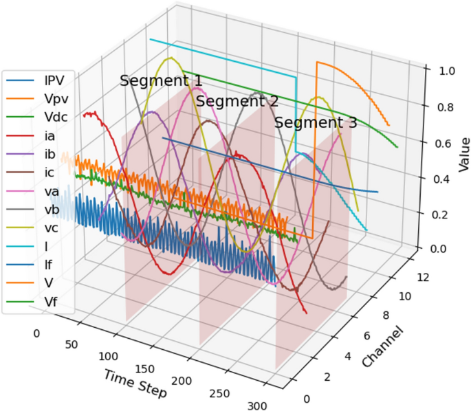
The scaled-segmented time series.
-
3.
Time–Frequency 2D Scalograms generation: CNNs are widely recognized for their ability to extract features from 2D images effectively. To leverage the strengths of pretrained CNN architectures like MobileNet 45, GoogleNet 46, and NASNetMobile 47, time series signals, typically presented in the time domain, can be transformed into Time–Frequency 2D scalograms using Continuous Wavelet Transform.
This transformation allows for the simultaneous analysis of signals in both the time and frequency domains, offering valuable insights into the underlying patterns. The mathematical formula of CWT is as follows:
$$CWT(a,b)=\frac{1}{\sqrt{a}}{\int }_{-\infty }^{+\infty }x\left(t\right){\psi }^{*}\left(\frac{t-b}{a}\right)dt$$(3)where, ψ(t) is the mother wavelet function, ψ(t) is shifted by b and delayed by a before its product with the time series signal x(t). In this study, we use the Morlet wavelet function with scales ranging from 1 to 32. Each of the generated grayscale scalograms represents a channel of the underlying time series data. These grayscale scalograms are then subjected to color mapping to generate RGB images, as shown in Figure 2.
Figure 2 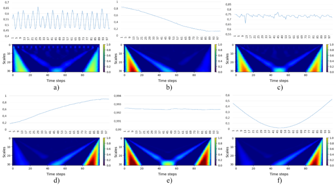
Examples of 2D scalograms: (a) Ipv in healthy case, (b) Ia in inverter fault, (c) Vpv in PV mismatch, (d) Ic in boost fault, (e) If in grid anomaly, (f) If in open circuit.
-
4.
Scalograms stacking: to consolidate the 13 scalograms generated for each sample into a single image, the next step involves stacking the scalograms vertically. This stacking preserves the temporal order of the original time series data while capturing multi-scale features extracted by the continuous wavelet transform.
Subsequently, the resulting composite images are then resized to dimensions of 224x224x3 pixels to align with the input specifications of pretrained architectures.


Methodology
In this study, four diagnosis methods suitable for low-cost edge devices for grid-connected PV systems have been investigated. These include GoogleNet InceptionV3, MobileNet, and NASNetMobile architectures, all of which were trained on the ImageNet database48, along with a developed lightweight 2D CNN architecture (LW-2DCNN).
It is important to note that the pretrained architectures have been specifically fine-tuned to handle 8 classes, ensuring their applicability to the diagnosis task at hand.
GoogLeNet InceptionV3 architecture
GoogleNet, also known as Inception, is a convolutional neural network architecture that achieved first place in the ILSVRC 2014 competition. The InceptionV3 network, a variant of the GoogLeNet architecture with 48 layers, is utilized for feature extraction. By leveraging factorized convolutions, such as 1 × 1 and 3 × 3 convolutions, InceptionV3 reduces the number of connections and parameters while maintaining efficiency. Furthermore, notable features of this architecture include the innovative integration of inception modules, which simultaneously utilize different filter sizes, enabling it to capture intricate patterns across multiple scales and hierarchies46 (see Fig. 3).

GoogleNet InceptionV3 architecture.
MobileNet architecture
MobileNetV1 is a lightweight CNN architecture proposed by researchers from Google in 2017. This architecture is developed to improve the deep learning performance under limited computational resources. MobileNet is based on depthwise (dw) separable convolutions which factorize a typical convolution layers into a depthwise convolution and pointwise convolutions to reduce computations and model size45 (see Fig. 4a).

Architecture of: (a) MobileNetV1, (b) NASNetMobile.
NASNetMobile architecture
The NASNetMobile architecture was introduced by researchers from Google in 201847. Based on the Neural Architecture Search (NAS) framework, NASNetMobile is designed to autonomously seek the optimal neural network architecture through reinforcement learning on a smaller dataset. Following this, the refined architecture is transferred to the extensive ImageNet dataset. NASNetMobile relies on depthwise separable convolutional layers, which consist of depthwise convolution followed by pointwise convolution. This architectural choice significantly reduces computational complexity while maintaining accuracy. Moreover, NASNetMobile is specifically tailored for devices with limited computational resources, offering a fine balance between computational efficiency and accuracy47 (see Fig. 4b).
Lightweight 2D-CNN (LW-2DCNN)
CNN structure
CNN is a feedforwad neural network based on convolutional architectures capable of capturing features without the need for manual intervention. Furthermore, this networks is characterized by adopting kernels that are sensitive to certain features. As a result, compared to traditional fully-connected structures, CNNs exhibit faster convergence and reduced number of parameters due to their effectiveness in preserving only useful data49. CNN can be composed of different layers:
-
Convolutional layer: the convolutional layer is a cornerstone in the design of CNNs. This layer is characterized by its convolutional filters (known as kernels) used to extract features from input images. In the early stages of a CNN, convolutional layers generate low-level feature maps, while later convolutional layers generate more complex feature maps, respectively50,51. The output feature map can be calculated as:
$$\widehat{{F}_{j}}={\sum }_{i}{F}_{i}\otimes {K}_{i,j}+{b}_{j}$$(4)where \({F}_{i}\) represents the ith feature map, \({K}_{i,j}\) is the kernel, \({b}_{j}\) is the bias, and \(\otimes\) is the 2-D convolution operation.
-
ReLU (Rectified Linear Unit) layer: the second layer incorporates non-linear factors to enhance the CNN’s fitting capabilities, achieved by using activation functions such as Sigmoid, Tanh, and ReLU. ReLU is often the preferred function due to its ease of implementation and its ability to transform all input values into positive numbers, thus reducing the computational demand51. The output of ReLU layer can be calculated as follows:
$$ReLU\left(x\right)=\left\{\begin{array}{c}x, \,\,\,\,\,\,\,\,if x>0\\ 0, \,\,\,\,\,\,\,\,otherwise\end{array}\right.$$(5) -
Pooling layer: as data progresses through the first layers, feature maps are generated. These maps, however, tend to be large, posing a potential risk of overfitting and leading to exhaustive calculations during the training process. To mitigate this, the introduction of a pooling layer is crucial. This layer downsamples the feature maps efficiently without losing the significant features. Commonly used methods include min pooling, max pooling, and global average pooling51.
-
Dropout layer: dropout is a widely employed regularization technique in neural networks. With this technique, a certain percentage of randomly selected neurons are “dropped out” during each training iteration. This process compels the network to rely on a diverse set of neurons and learn from less data, thereby enhancing its ability to generalize. Dropout mitigates overfitting, by encouraging the learning of more robust features, and improves the model’s generalization capabilities52,53.
-
Fully-connected layer: the fully-connected layers are employed at the end of the CNN, where the output of the last pooling layer is fed to these layers to be flattened before being delivered to the classifier. Subsequently, the SoftMax activation function is used in the last layer to calculate the probability values of the classes54.
Design of lightweight CNN
-
Energy valley optimizer: Mahdi et al. 55 proposed the energy valley optimizer imitating the cutting-edge physics principles regarding particles’ stability and different modes of decay as exposed in Fig. 5. The vast majority of particles existing in the universe are considered unstable. To achieve stability, these particles tend to release energy through decay process including alpha, beta, gamma, electron capture (EC), and/or positron emission (PE), wherein a lower-energy particle is produced as the extra energy is discharged. Lighter particles with neutron-to-proton ratio N/Z ≈ 1 often exhibits stability, while for heavier particle, the stability band tends to shift slightly towards higher N/Z ratio.
Figure 5 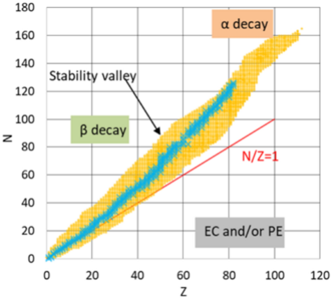
Stability valley for particles.

-
1.
Initialization process
-
Particles (Xi): are random particles in the search space as follows:
$$X=\left[\begin{array}{c}{x}_{1}^{1}{x}_{1}^{2}\dots {x}_{1}^{j}\dots {x}_{1}^{d}\\ {x}_{2}^{1}{x}_{2}^{2}\dots {x}_{2}^{j}\dots {x}_{2}^{d}\\ \vdots \\ {x}_{i}^{1}{x}_{i}^{2}\dots {x}_{i}^{j}\dots {x}_{i}^{d}\\ {x}_{n}^{1}{x}_{n}^{2}\dots {x}_{n}^{j}\dots {x}_{n}^{d}\end{array}\right],\left\{\begin{array}{c}i=\text{1,2},\dots n\\ j=\text{1,2},\dots d\end{array}\right.$$(6)where n is the total number of particles in the search space and d is the dimension of the considered problem.
-
Enrichment bound of particles (EB): the Enrichment Bound of the particles is used to distinguish between neutron-rich and neutron-poor particles. It can be calculated as follows:
$$EB=\frac{\sum_{i=1}^{n}{NEL}_{i}}{n}$$(7)where \({NEL}_{i}\) is the Neutron Enrichment Level of ith particle (the score of ith particle).
-
Stability Levels of the particles (SL): the stability levels of the particles are determined as follows:
$${SL}_{i}=\frac{{NEL}_{i}-BS}{WS-BS}$$(8)where \({SL}_{i}\) is the stability level of the ith particle, BS and WS is are the particles with best and worst stability levels equivalent to the minimum and maximum scores.
-
2.
Decay process
-
Alpha decay: Alpha decay occurs when the neutron enrichment level of a particle exceeds the enrichment bound, and the stability level (SL) of a particle surpasses the stability bound (SB). This typically happens with heavier particles having a larger neutron-to-proton (N/Z) ratio. This can be denoted as (\({NEL}_{i}>EB\)) & (\({SL}_{i}>SB\)) and can be mathematically described as a new solution candidate and it is generated as follows:
$${X}_{i}^{new1}{=X}_{i}\left({X}_{BS}\left({X}_{i}^{j}\right)\right), j=ALpha Index II$$(9)where \({X}_{i}^{new1}\) is the generated particle, \({X}_{i}\) is the current position vector of the ith particle, \({X}_{BS}\) is the position vector of the particle with the best stability level, \({X}_{i}^{j}\) is the jth emitted ray, Alpha Index I in the range of [1, d], which mimics the number of emitted rays, and Alpha Index II in the range of [1, Alpha Index I], which mimics which alpha rays to be emitted.
-
Gamma decay: Gamma rays are emitted from the same particles that undergo alpha decay. A neighboring particle replaces the photons within the excited particles. This can be expressed as:
$${X}_{i}^{new2}{=X}_{i}\left({X}_{Ng}\left({X}_{i}^{j}\right)\right), j=Gamma Index II$$(10)where \({X}_{Ng}\) is the position vector of the neighboring particle, Gamma Index I in the range of [1, d] and Gamma Index II in the range of [1, Gamma Index I] are the number of emitted photons, and the photons to be emitted in the particle respectively. The neighboring particle can be selected according to the following distance:
$${D}_{i}^{k}=\sqrt{{{(x}_{2}-{x}_{1})}^{2}+{{(y}_{2}-{y}_{1})}^{2}}, k=\text{1,2},\dots ,n-1$$(11)where \({D}_{i}^{k}\) is the total distance between the ith particle and the kth neighboring particle, and (\({x}_{1}\), \({y}_{1}\)) and (\({x}_{2}\), \({y}_{2}\)) are the coordinates of the particles.
-
Beta decay: this decay is exhibited by unstable particles with lower SL (\({SL}_{i}\le SB\)). In this decay, a significant jump is expected because of the higher instability of this type of particles. Therefore, a movements toward the particle with the best stability level \({X}_{BS}\), the centre of particles \({X}_{CB}\), and the neighboring particle \({X}_{Ng}\) are formulated as follows:
$${X}_{CP}=\frac{\sum_{i=1}^{n}{X}_{i}}{n}$$(12)$${X}_{i}^{new1}={X}_{i}+\frac{({r}_{1}*{X}_{BS}-{r}_{2}*{X}_{CP})}{{SL}_{i}}$$(13)$${X}_{i}^{new2}={X}_{i}+({r}_{3}*{X}_{BS}-{r}_{4}*{X}_{Ng})$$(14)where, (\({r}_{1}\), \({r}_{2}\), \({r}_{3}\), and \({r}_{4}\)) are random numbers in the range of [0, 1] which determine the movements of particles.
-
Electron capture EC and/or positron emission PE: this process is exhibited by particles with a smaller N/Z ratio where (\({NLL}_{i}\le EB\)). A random movement is conducted as follows:
$${X}_{i}^{new}={X}_{i}+r$$(15)where \({X}_{i}^{new}\) the upcoming position and \(r\) is a random number in the range of [0, 1]42.
-
CNN parameters optimization: Fine-tuning CNN hyperparameters can be a laborious and time-consuming task. Typically, the trial-and-error approach is employed to select the optimal combination of hyperparameters. In this study, we employed a systematic approach to fine-tune the hyperparameters of LW-2DCNN, aiming to optimize performance across grid-connected photovoltaic system fault diagnosis scenarios. We utilized the energy valley optimizer, a metaheuristic optimization technique known for its effectiveness in handling complex parameter spaces, with the training parameters listed in Table 4. The ranges were carefully selected to balance model complexity and optimize performance, taking into account the computational limitations of low-cost edge devices. By focusing on narrow ranges, we aimed to identify configurations that maximize predictive accuracy while minimizing computational overhead.
Table 4 Training parameters used in EV optimizer.
Applying the optimizer to the entire dataset is however computationally expensive. Therefore, 10% of the dataset is used for optimization. The optimization algorithm is run for 10 iterations, conducting searches in a 7-dimensional search domain. The optimizer explores a continuous search domain and produces continuous values during optimization. These values are converted into discrete values by rounding them to the nearest integer. The score of particles is evaluated using the training/validation accuracies and losses as follows:
Figure 6 shows the convergence curve of EVO particles. Initially, the particles are scattered randomly in the search space. As the optimization progresses, particles move towards more promising regions (towards the stability valley). After the 5th iteration, the convergence curve flattens out, indicating that the particles converge towards the best solution in the search space. The hyperparameters considered in this study, their corresponding ranges, and optimized values are outlined in Table 5. The architecture and detailed parameters of optimized LW-2DCNN are illustrated in Figure. 7 and Table 6 respectively. The detailed flowchart of the developed fault diagnosis technique is illustrated in Figure 8.

Particles score curve.

Architecture of LW-2DCNN.

Detailed flowchart of the proposed fault diagnosis approach.
Performance metrics
The developed diagnosis approach is quantitatively evaluated in terms of five criteria (Accuracy (Acc), Precision (Pr), Sensitivity (Sn), Specificity (Sp), and F1-score (F1)).
-
Accuracy: this metric provides an overall measure of how well the model correctly identifies both faulty and non-faulty instances within the dataset. This metric is a fundamental measure of the model’s overall performance. It can be described as follows:
$$Acc=\frac{TP+TN}{TP+TN+FP+FN}100\%$$(17)where, TP is the True Positive, TN is the True Negative, FP is the false Positive, and FN is the False Negative.
-
Precision: it measures the proportion of true positive predictions out of all positive predictions made by the diagnosis model. In the context of fault detection, precision is crucial for ensuring that maintenance actions are targeted and cost-effective. The precision can be calculated as:
$$Pr=\frac{TP}{TP+FP}100\%$$(18) -
Sensitivity: also known as recall, it measures the proportion of true positives that are correctly identified by the model. This metric is important in fault detection scenarios to ensure that all true positives (actual faults) are correctly detected and addressed, thereby minimizing the risk of system failures. It can be calculated as :
$$Sn=\frac{TP}{TP+FN}100\%$$(19) -
Specificity: it measures the proportion of true negatives that are correctly identified by the model. It complements sensitivity by ensuring that healthy instances are accurately classified as such, thereby reducing unnecessary maintenance interventions. Specificity can be calculated as:
$$Sp=\frac{TN}{TN+FP}100\%$$(20) -
F1-score: is the harmonic mean of precision and sensitivity, providing a balanced measure that considers both false positives and false negatives. It is useful in case of unbalanced dataset scenarios. This metric can be determined as:
$$F1=\frac{2*TP}{2*TP+FP+FN}100\%$$(21)
Results and discussion
To validate the performance of the proposed detection and diagnostic approach, two classification tasks are conducted. The first task involves binary fault classification using an augmented large dataset. The second task comprises multi-fault classification, which includes three case studies: one with a balanced dataset distribution, another with an unbalanced dataset distribution, and a third with a noise effect. The evaluation is conducted through comparisons with well-established architectures such as MobileNet, NASNetMobile, and InceptionV3 as well as with existing studies in the literature.
The diagnosis methods are implemented using Python programming language and are run on a computer with the configuration: Intel (R) Core (TM) i5-4210U CPU @ 1.70 GHz, 8 GB (RAM), 64 bits.
Binary classification (Fault detection)
In this test, a binary classification task is conducted to showcase the effectiveness of the proposed Continuous Wavelet Transform-based visualization approach that converts raw 1D data into 2D images. Additionally, the original data of the healthy class is augmented by applying a time shift to preserve temporal information. The abnormal class comprises a mix of 7 faults. The detailed description of the dataset used is highlighted in Table 7.
This augmentation aims to balance the dataset and evaluate the scalability of the proposed processing method. To ensure a fair comparison, two baseline Convolutional Neural Network models with the same structure are implemented. The first is a 1D CNN model used for classifying the 1D data, and the second is a 2D CNN model used for classifying the 2D images. The detailed structure of the baseline models is provided in Table 8.
Figure 9 shows the training accuracy and loss of the baseline 1D and 2D CNN models. Clearly, the accuracy curve of the 2D-CNN model converges rapidly, whereas the accuracy of the 1D-CNN model converges more slowly and exhibits higher fluctuations. Similarly, the loss curve of the 2D-CNN model approaches zero after a few iterations, despite an initially high loss. In contrast, the loss of the 1D-CNN model decreases over iterations but converges more slowly.

(a) Accuracy of training phase, (b) Loss of training phase.
The confusion matrices of the baseline models shown in Fig. 10 clearly demonstrate that the 2D-CNN model outperforms the 1D-CNN model in identifying healthy samples and detecting abnormal samples. The 2D-CNN model accurately identified 631 out of 634 healthy class images and detected 610 out of 638 abnormal class images. In contrast, the 1D-CNN model correctly identified 601 out of 634 healthy samples and detected 602 out of 638 abnormal samples, indicating lower overall performance. The overall comparison of the two baseline models across selected performance criteria demonstrates that the 2D-CNN model exhibits superior performance compared to the 1D-CNN model as highlighted in Table 9.

Confusion matrices of: (a) 2D-CNN, (b) 1D-CNN.
Multi-class classification (Fault diagnosis)
In this case study, a multi-class classification task is performed. The dataset, comprising 8 classes (1 healthy and 7 faulty), is down-sampled to test our diagnostic approach against a small dataset and to verify its suitability for resource-constrained environments. The detailed down-sampled dataset is presented in Table 10.
Balanced dataset distribution
In this evaluation phase, the diagnosis methods are assessed using a balanced dataset containing classes of equal size, as depicted in Fig. 11a. The dataset comprises a total of 4800 images, which are allocated as follows: 70% for training and the remaining 30% equally split between validation and testing, with 720 images each. The batch size is 32, the maximum number of epochs is set to 50 (5250 iterations). The model loss function is minimized using ‘Adam’ optimizer with a learning rate chosen as 5e−5. The training accuracy of MobileNet, NASNetMobile, InceptionV3, and LW-2DCNN is presented in Fig. 12a. The training accuracy of LW-2DCNN (curve in green) reached saturation within 10 epochs with fewer batch accuracy fluctuations compared to MobileNet (curve in blue), NASNetMobile (curve in brown), and InceptionV3 (curve in red) which exhibit slower convergence and higher batch accuracy fluctuations. LW-2DCNN achieved a training convergence of 100%. While MobileNet, NASNetMobile, and InceptionV3 reached 80%, 90%, and 96% respectively. Moreover, the training loss of LW-2DCNN converges to 0.007 after only 10 epochs, while the MobileNet, NASNetMobile, and InceptionV3 architectures reached losses of 1.32, 1.29, and 0.78 respectively after 50 epochs as shown in Fig. 12b.

Dataset distributions of: (a) balanced scenario, (b) unbalanced scenario.

(a) Accuracy of training phase, (b) Loss of training phase.
The confusion matrices for MobileNet, NASNetMobile, InceptionV3 and LW-2DCNN are depicted in Fig. 13. As observed, MobileNet model predicted 583 out of 720, NASNetMobile predicted 636 out of 720, while InceptionV3 model correctly predicted 706 out of 720 samples. Conversely, the designed model successfully predicted 100% of the test images across all eight classes. The classification report for the diagnosis methods under a balanced dataset distribution is presented in Table 11. It is evident that the proposed LW-2DCNN outperforms MobileNet, NASNetMobile and InceptionV3. Notably, the accuracy, precision, sensitivity, specificity, and F1 score all achieve 100%.

Confusion matrices of balanced dataset: (a) MobileNet, (b) NASNetMobile, (c) InceptionV3, and (d) LW-2DCNN.
Unbalanced dataset distribution
In this section, we present the results of the diagnosis methods on an unbalanced dataset distribution. The unbalanced dataset is distributed as follows, 81 images for the healthy case, 54 images for IGBT fault, 76 images for Sensor fault, 67 images for grid anomaly, 117 images for mismatch, 99 images for OC fault, 126 images for MPPT fault, and 99 images for boost converter fault. The distribution of the 8 classes is shown in Fig. 11b. The confusion matrices of the diagnosis methods and the comprehensive report are shown in Fig. 14 and Table 12 respectively. As can be seen, the performance of all three diagnosis methods is impacted by the unbalanced dataset distribution. However, LW-2DCNN exhibits a comparatively lower performance degradation (< 0.5% for all matrices) compared to MobileNet, NASNetMOBILE, and InceptionV3.

Confusion matrices of unbalanced dataset: (a) MobileNet, (b) NASNetMobile, (c) InceptionV3, and (d) LW-2DCNN.
Noisy dataset
In this scenario, the diagnostic methods are tested on a noisy dataset to simulate real-world scenarios where the collected dataset is subject to various types of noise, such as sensor inaccuracies and measurement errors. To achieve this, white noise is added to the 1D time series dataset using a Gaussian distribution as follows:
where, \(\widehat{D}\) and \(D\) are the noisy and noiseless datasets respectively, f is noise term, \(\mu =0\) and \(\sigma =0.1\) are the mean and the standard deviation of the normal distribution respectively. The performance of the diagnosis methods on the noisy dataset is deteriorated, as summarized in Table 13. It is evident that LW-2DCNN, although affected by noise, demonstrates the least reduction in performance, decreasing from an accuracy of 100% to 93.75%. This observation underscores its effectiveness in mitigating the impact of noise. Moreover, the confusion matrices of MobileNet, InceptionV3, and LW-2DCNN are illustrated in Fig. 15. In the case of MobileNet, out of 720 test images, 294 were correctly predicted. NASNetMobile and InceptionV3 achieved performances close to MobileNet with 303 and 263 correct predictions out of 720 images respectively. Notably, the LW-2DCNN model successfully predicted 675 out of 720 test images with 93.75% accuracy.

Confusion matrices of noisy dataset: (a) MobileNet, (b) NASNetMobile, (c) InceptionV3, and (d) LW-2DCNN.
Figure 16 presents the distributions of extracted features from the all four diagnosis methods under balanced, unbalanced, and noisy datasets, visualized using t-distributed stochastic neighbor embedding (t-SNE). For the balanced dataset case shown in in the first row, it can be observed that the clusters corresponding to the faults are relatively tight for all four methods, indicating clear separability. However, LW-2DCNN exhibits more compact and well-defined clusters compared to MobileNet, NASNetMobile, and InceptionV3. In the second row, representing the unbalanced dataset, the clusters remain generally separable for LW-2DCNN. However, there is slightly more overlap between classes observed for other architectures. In the third row, depicting the noisy dataset, LW-2DCNN maintains cluster separability despite some small overlap. In contrast, MobileNet, NASNetMoble, and InceptionV3 exhibit significant overlap, with no distinct boundaries between clusters. This suggests that they struggle to capture the discriminative information necessary for distinguishing between classes effectively.

t-SNE of MobileNet, NASNetMobile, InceptionV3, and LW-2DCNN of: (a) balanced, (b) unbalanced, (c) noisy dataset scenarios.
Discussion and limitations of the study
The early fault detection and diagnosis in grid-connected PV systems are essential to maintain their stability and reliability. Deep learning techniques, notably convolutional neural networks, have demonstrated remarkable performance, particularly in classifying 2D image data. However, when dealing with 1D time series signals common in PV system monitoring, leveraging CNNs can be challenging. To address this, researchers have turned to visualizing time series approaches like continuous wavelet transform to exploit CNN capabilities and employ pretrained architectures. Moreover, there is a growing interest in investigating lightweight CNN architectures for monitoring and diagnosis algorithms to be used on low-cost edge devices.
In this article, we propose an effective diagnosis approach for grid-connected PV faults based on a lightweight 2D CNN optimized by the Energy Valley Optimization algorithm. The input 1D signals are visualized using a CWT-based approach. The proposed architecture is compared with well-established benchmarks, namely MobileNet, NASNetMobile, and InceptionV3 pretrained architectures. These models are renowned for their effectiveness while being optimized for efficiency in terms of computational resources.
The comparison results, including balanced, unbalanced, and noisy datasets, as well as training time and the number of parameters, are depicted in Fig. 17. As is evident, the diagnosis accuracy of the proposed LW-2DCNN outperforms MobileNet, NASNetMobile, and InceptionV3 architectures in all test scenarios with an accuracy of 97.87% (averaged over the three test scenarios). For the training duration, the proposed CNN achieved convergence in a shorter time frame (85 min) compared to 133 min for MobileNet, 276 min for NASNetMobile, and 228 min for InceptionV3. This can be attributed to the well-selected parameters using the Energy Valley optimizer.

Overall performance comparison.
Moreover, in terms of the number of parameters, the proposed LW-2DCNN demonstrates a substantial reduction, with 6 times fewer parameters compared to InceptionV3. Although it is slightly larger (by only 0.4%) compared to MobileNet, this marginal increase can be overlooked given the superior performance of the LW-2DCNN. Furthermore, the proposed diagnosis method is compared to previous similar methods in the literature that use Continuous Wavelet Transform to visualize 1D time series. Table 14 presents a detailed comparison of PV fault diagnosis methods in terms of the year of publication, diagnosis technique, number of classes, test scenarios, test accuracy, and number of parameters.
In32, two PV fault diagnosis approaches based on fine-tuned pretrained AlexNet models are proposed. Despite the use of heavy architecture, which comprises 60 million parameters, the best obtained accuracy is modest at 73.53%. In40, a fault diagnosis method based on light CNN architecture for microgrids is introduced, achieving a notable accuracy of 97.12%. However, this method only addresses short-circuit faults. In36, a ConvMixer is utilized to diagnose the detected faults, using the Markov transition field transform to generate images. Despite the small number of parameters in this model, it is validated only under unbalanced dataset conditions. In41, a method for detecting partial shading based on fine-tuned AlexNet is presented, achieving an accuracy of 98.05%. However, it’s worth mentioning that this method exclusively detects partial shading anomalies and is tested solely on balanced dataset scenarios. The proposed diagnosis models in43 and14 showed good performance with a relatively small number of parameters. However, they focused on physical faults and did not address parametric faults. Therefore, based on the above quantitative analysis, it can be said that the proposed method showcased remarkably improved performance in classification accuracies, achieving 100%, 99.86%, and 93.75% for balanced, unbalanced, and noisy datasets respectively. Notably, these results were attained despite the relatively low number of parameters and short training time of the proposed method, rendering it well-suited for deployment on low-cost edge devices.
Our study’s findings hold significant implications for real-world applications in grid-connected photovoltaic (PV) systems. They enhance fault diagnosis accuracy, operational efficiency, and scalability, contributing to maintaining PV systems reliability, reducing downtime, and optimizing maintenance schedules. The integration of our approach facilitates real-time fault detection and diagnosis, enabling prompt responses to system anomalies. This capability supports sustainable energy management practices and ensures uninterrupted power supply in diverse operational conditions.
While the method demonstrates effectiveness in detecting and classifying individual faults in grid-connected PV systems, its applicability to scenarios involving mixed faults has not been explored. Furthermore, the current study does not address online fault detection capabilities. Future research could focus on extending the method to handle mixed faults and incorporating online fault detection, thereby significantly enhancing its practical utility in real-world applications.
Conclusion
In this study, a diagnosis technique for faults in grid-connected PV systems is introduced. The method relies on a lightweight two-dimensional convolutional neural network. Initially, the collected 1D time series signals are visualized using continuous wavelet transform to harness the capabilities of CNNs in computer vision. Subsequently, the proposed architecture is fine-tuned using the Energy Valley optimizer. Obtained results indicate that the proposed diagnosis method is effective in fault classification, achieving higher test accuracies of up to 100%, 99.86%, and 93.75% across balanced, unbalanced, and noisy datasets, respectively, compared to other well-established architectures such as MobileNet, NASNetMobile, and InceptionV3, as well as similar studies in the literature. Additionally, the proposed method demonstrates shorter training durations and a relatively small number of parameters, further highlighting its efficiency and, practicality, and suitability for low-cost edge devices.
Data availability
The datasets used and/or analysed during the current study available from the corresponding author on reasonable request.
References
Paramati, S. R., Shahzad, U. & Doğan, B. The role of environmental technology for energy demand and energy efficiency: Evidence from OECD countries. Renew. Sustain. Energy Rev. 153, 111735. https://doi.org/10.1016/j.rser.2021.111735 (2022).
Kober, T. et al. Global energy perspectives to 2060–WEC’s World Energy Scenarios 2019. Energ. Strat. Rev. 31, 100523. https://doi.org/10.1016/j.esr.2020.100523 (2020).
Bhattarai, U., Maraseni, T. & Apan, A. Assay of renewable energy transition: A systematic literature review. Sci. Total Environ. 833, 155159. https://doi.org/10.1016/j.scitotenv.2022.155159 (2022).
Kijo-Kleczkowska, A., Bruś, P. & Więciorkowski, G. Profitability analysis of a photovoltaic installation: A case study. Energy 261, 125310. https://doi.org/10.1016/j.energy.2022.125310 (2022).
Ahmad, M., Dai, J., Mehmood, U. & Abou, Houran M. Renewable energy transition, resource richness, economic growth, and environmental quality: Assessing the role of financial globalization. Renew. Energy 216, 119000. https://doi.org/10.1016/j.renene.2023.119000 (2023).
Greim, P., Solomon, A. A. & Breyer, C. Assessment of lithium criticality in the global energy transition and addressing policy gaps in transportation. Nat. Commun. 11(1), 4570. https://doi.org/10.1038/s41467-020-18402-y (2020).
Xie, P. & Jamaani, F. Does green innovation, energy productivity and environmental taxes limit carbon emissions in developed economies: Implications for sustainable development. Struct. Change Econ. Dyn. 63, 66–78. https://doi.org/10.1016/j.strueco.2022.09.002 (2022).
Nagarajan, K. et al. Optimizing dynamic economic dispatch through an enhanced Cheetah-inspired algorithm for integrated renewable energy and demand-side management. Sci. Rep. 14(1), 3091. https://doi.org/10.1038/s41598-024-53688-8 (2024).
Korkmaz, D. & Acikgoz, H. An efficient fault classification method in solar photovoltaic modules using transfer learning and multi-scale convolutional neural network. Eng. Appl. Artif. Intell. 113, 104959. https://doi.org/10.1016/j.engappai.2022.104959 (2022).
Mustafa, Z., Awad, A. S., Azzouz, M. & Azab, A. Fault identification for photovoltaic systems using a multi-output deep learning approach. Exp. Syst. Appl. 211, 118551. https://doi.org/10.1016/j.eswa.2022.118551 (2023).
IRENA (2023), Renewable energy statistics 2023, International Renewable Energy Agency, Abu Dhabi. https://mc-cd8320d4-36a1-40ac-83cc-3389-cdn-endpoint.azureedge.net/ /media/Files/IRENA/Agency/Publication/2023/Jul/IRENA_Renewable_energy_statistics_2023.pdf?rev=7b2f44c294b84cad9a27fc24949d2134
Amiri, A., Samet, H. & Ghanbari, T. Recurrence plots based method for detecting series arc faults in photovoltaic systems. IEEE Transact. Indus. Electron. 69(6), 6308–15. https://doi.org/10.1109/TIE.2021.3095819 (2021).
Mellit, A., Tina, G. M. & Kalogirou, S. A. Fault detection and diagnosis methods for photovoltaic systems: A review. Renew. Sustain. Energy Rev. 91, 1–7. https://doi.org/10.1016/j.rser.2018.03.062 (2018).
Hong, Y. Y. & Pula, R. A. Diagnosis of photovoltaic faults using digital twin and PSO-optimized shifted window transformer. Appl. Soft Comput. 150, 111092. https://doi.org/10.1016/j.asoc.2023.111092 (2024).
Wang, J., Gao, D., Zhu, S., Wang, S. & Liu, H. Fault diagnosis method of photovoltaic array based on support vector machine. Energy Sour. Part a Recov. Util. Environ. Eff. 45(2), 5380–95. https://doi.org/10.1080/15567036.2019.1671557 (2023).
Ladel, A. A., Outbib, R., Benzaouia, A., Ouladsine, M. Simultaneous switched model-based fault detection and MPPT for photovoltaic systems. In: 2022 10th International Conference on Systems and Control (ICSC). IEEE, 2022. p. 410-415. https://doi.org/10.1109/ICSC57768.2022.9993833
Bouyeddou, B., Harrou, F., Taghezouit, B., Sun, Y. & Hadj, Arab A. Improved semi-supervised data-mining-based schemes for fault detection in a grid-connected photovoltaic system. Energies 15(21), 7978. https://doi.org/10.3390/en15217978 (2022).
El-Banby, G. M., Moawad, N. M., Abouzalm, B. A., Abouzaid, W. F. & Ramadan, E. A. Photovoltaic system fault detection techniques: A review. Neural Comput. Appl. 35(35), 24829–42. https://doi.org/10.1007/s00521-023-09041-7 (2023).
Bakdi, A., Bounoua, W., Guichi, A. & Mekhilef, S. Real-time fault detection in PV systems under MPPT using PMU and high-frequency multi-sensor data through online PCA-KDE-based multivariate KL divergence. Int. J. Electr. Power Energy Syst. 125, 106457. https://doi.org/10.1016/j.ijepes.2020.106457 (2021).
Tsanakas, J. A., Ha, L. & Buerhop, C. Faults and infrared thermographic diagnosis in operating c-Si photovoltaic modules: A review of research and future challenges. Renew. Sustain. Energy Rev. 62, 695–709. https://doi.org/10.1016/j.rser.2016.04.079 (2016).
Herraiz, Á. H., Marugán, A. P. & Márquez, F. P. Photovoltaic plant condition monitoring using thermal images analysis by convolutional neural network-based structure. Renew. Energy 153, 334–48. https://doi.org/10.1016/j.renene.2020.01.148 (2020).
Sizkouhi, A. M., Aghaei, M. & Esmailifar, S. M. A deep convolutional encoder-decoder architecture for autonomous fault detection of PV plants using multi-copters. Sol. Energy 223, 217–28. https://doi.org/10.1016/j.solener.2021.05.029 (2021).
Gu, J. C., Lai, D. S., Wang, J. M., Huang, J. J. & Yang, M. T. Design of a DC series arc fault detector for photovoltaic system protection. IEEE Trans. Indus. Appl. 55(3), 2464–71. https://doi.org/10.1109/TIA.2019.2894992 (2019).
Li, B., Delpha, C., Migan-Dubois, A. & Diallo, D. Fault diagnosis of photovoltaic panels using full I-V characteristics and machine learning techniques. Energy Convers. Manag. 248, 114785. https://doi.org/10.1016/j.enconman.2021.114785 (2021).
Mellit, A. & Kalogirou, S. Artificial intelligence and internet of things to improve efficacy of diagnosis and remote sensing of solar photovoltaic systems: Challenges, recommendations and future directions. Renew. Sustain. Energy Rev. 143, 110889. https://doi.org/10.1016/j.rser.2021.110889 (2021).
Amiri, A. F., Oudira, H., Chouder, A. & Kichou, S. Faults detection and diagnosis of PV systems based on machine learning approach using random forest classifier. Energy Convers. Manag. 301, 118076. https://doi.org/10.1016/j.enconman.2024.118076 (2024).
Yu, W., Liu, G., Zhu, L. & Yu, W. Convolutional neural network with feature reconstruction for monitoring mismatched photovoltaic systems. Sol. Energy 212, 169–77. https://doi.org/10.1016/j.solener.2020.09.026 (2020).
Khan, K. et al. Data-driven green energy extraction: Machine learning-based MPPT control with efficient fault detection method for the hybrid PV-TEG system. Energy Rep. 9, 3604–23. https://doi.org/10.1016/j.egyr.2023.02.047 (2023).
Chen, Z., Chen, Y., Wu, L., Cheng, S. & Lin, P. Deep residual network based fault detection and diagnosis of photovoltaic arrays using current-voltage curves and ambient conditions. Energy Convers. Manag. 198, 111793. https://doi.org/10.1016/j.enconman.2019.111793 (2019).
Chen, S., Yu, J. & Wang, S. One-dimensional convolutional auto-encoder-based feature learning for fault diagnosis of multivariate processes. J. Process Control 87, 54–67. https://doi.org/10.1016/j.jprocont.2020.01.004 (2020).
Gao, W. & Wai, R. J. A novel fault identification method for photovoltaic array via convolutional neural network and residual gated recurrent unit. IEEE Access 8, 159493–510. https://doi.org/10.1109/ACCESS.2020.3020296 (2020).
Aziz, F. et al. A novel convolutional neural network-based approach for fault classification in photovoltaic arrays. IEEE Access 8, 41889–904. https://doi.org/10.1109/ACCESS.2020.2977116 (2020).
Lu, X. et al. Fault diagnosis for photovoltaic array based on convolutional neural network and electrical time series graph. Energy Convers. Manag. 196, 950–65. https://doi.org/10.1016/j.enconman.2019.06.062 (2019).
Lu, S., Sirojan, T., Phung, B. T., Zhang, D. & Ambikairajah, E. DA-DCGAN: An effective methodology for DC series arc fault diagnosis in photovoltaic systems. IEEE Access 7, 45831–40. https://doi.org/10.1109/ACCESS.2019.2909267 (2019).
Liu, G., Zhu, L., Yu, W. & Yu, W. Image formation, deep learning, and physical implication of multiple time-series one-dimensional signals: Method and application. IEEE Trans. Indus. Inf. 17(7), 4566–74 (2020).
Hong, Y. Y. & Pula, R. A. Diagnosis of PV faults using digital twin and convolutional mixer with LoRa notification system. Energy Rep. 9, 1963–76. https://doi.org/10.1016/j.egyr.2023.01.011 (2023).
Korkmaz, D. & Acikgoz, H. An efficient fault classification method in solar photovoltaic modules using transfer learning and multi-scale convolutional neural network. Eng. Appl. Artif. Intell. 113, 104959. https://doi.org/10.1016/j.engappai.2022.104959 (2022).
Lin, P. et al. Compound fault diagnosis model for Photovoltaic array using multi-scale SE-ResNet. Sustain. Energy Technol. Assess. 50, 101785. https://doi.org/10.1016/j.seta.2021.101785 (2022).
Kellil, N., Aissat, A. & Mellit, A. Fault diagnosis of photovoltaic modules using deep neural networks and infrared images under Algerian climatic conditions. Energy 263, 125902. https://doi.org/10.1016/j.energy.2022.125902 (2023).
Pan, P., Mandal, R. K. & Redoy AkandaRahman, M. M. Fault classification with convolutional neural networks for microgrid systems. Int. Trans. Electr. Energy Syst. 20(1), 8431450. https://doi.org/10.1155/2022/8431450 (2022).
Latoui, A. & Daachi, M. E. Real-time monitoring of partial shading in large PV plants using Convolutional Neural Network. Sol. Energy 253, 428–38. https://doi.org/10.1016/j.solener.2023.02.041 (2023).
Qu, J., Sun, Q., Qian, Z., Wei, L. & Zareipour, H. Fault diagnosis for PV arrays considering dust impact based on transformed graphical features of characteristic curves and convolutional neural network with CBAM modules. Appl. Energy 355, 122252. https://doi.org/10.1016/j.apenergy.2023.122252 (2024).
Gong, B., An, A., Shi, Y. & Zhang, X. Fast fault detection method for photovoltaic arrays with adaptive deep multiscale feature enhancement. Appl. Energy 353, 122071. https://doi.org/10.1016/j.apenergy.2023.122071 (2024).
Bakdi, A., Guichi, A., Mekhilef, S. & Bounoua, W. GPVS-Faults: Experimental Data for fault scenarios in grid-connected PV systems under MPPT and IPPT modes. Mendeley https://doi.org/10.17632/n76t439f65.1 (2020).
Howard, A. G. et al. Mobilenets: Efficient convolutional neural networks for mobile vision applications. arX. Prepr. arX. https://doi.org/10.48550/arXiv.1704.04861 (2017).
Szegedy, C., Liu, W., Jia, Y., Sermanet, P., Reed, S., Anguelov, D., Erhan, D., Vanhoucke, V., Rabinovich, A. Going deeper with convolutions. In Proceedings of the IEEE conference on computer vision and pattern recognition 2015 https://doi.org/10.48550/arXiv.1409.4842
Zoph, B., Vasudevan, V., Shlens, J., Le, Q. V. Learning transferable architectures for scalable image recognition. In Proceedings of the IEEE conference on computer vision and pattern recognition 2018 (pp. 8697-8710). https://doi.org/10.48550/arXiv.1707.07012
Deng, J. et al. Imagenet: A large-scale hierarchical image database. IEEE Conf. Comput. Vis. Pattern Recognit. 2009, 248–255 (2009).
Li, Z., Liu, F., Yang, W., Peng, S. & Zhou, J. A survey of convolutional neural networks: Analysis, applications, and prospects. IEEE Trans. Neural Netw. Learn. Syst. 33(12), 6999–7019. https://doi.org/10.1109/TNNLS.2021.3084827 (2021).
Ayadi, W., Elhamzi, W., Charfi, I. & Atri, M. Deep CNN for brain tumor classification. Neural Process. Lett. 53(1), 671–700. https://doi.org/10.1007/s11063-020-10398-2 (2021).
Alzubaidi, L. et al. Review of deep learning: Concepts, CNN architectures, challenges, applications, future directions. J. Big Data 8, 1–74. https://doi.org/10.1186/s40537-021-00444-8 (2021).
Wang, M. H., Hung, C. C., Lu, S. D., Lin, Z. H. & Kuo, C. C. Fault diagnosis for PV modules based on alexnet and symmetrized dot pattern. Energies 16(22), 7563. https://doi.org/10.3390/en16227563 (2023).
Dileep, P., Das, D., Bora, P. K. Dense layer dropout based CNN architecture for automatic modulation classification. In 2020 National conference on communications (NCC) 2020 Feb 21 (pp. 1–5). IEEE. https://doi.org/10.1109/NCC48643.2020.9055989
Memon, S. A. et al. A machine-learning-based robust classification method for PV panel faults. Sensors 22(21), 8515. https://doi.org/10.3390/s22218515 (2022).
Azizi, M., Aickelin, U., Khorshidi, H. A. & Baghalzadeh, S. M. Energy valley optimizer: A novel metaheuristic algorithm for global and engineering optimization. Sci. Rep. 13(1), 226. https://doi.org/10.1038/s41598-022-27344-y (2023).
Acknowledgements
The authors extend their appreciation to Taif University, Saudi Arabia, for supporting this work through the project number (TU-DSPP-2024-14).
Funding
This research was funded by Taif University, Taif, Saudi Arabia (TU-DSPP-2024-14).
Author information
Authors and Affiliations
Contributions
A.T.: Methodology, Data preparation, Software, Coding, Validation, Writing—Original draft. B.K.: Methodology, Reviewing and Editing. D.B.: Methodology, Reviewing and Editing. N.H.: Conceptualization, Reviewing and Editing. A.R.: Methodology, Software. M.A.: Reviewing and Editing, Supervision. M.B.: Reviewing and Editing, Validation, Supervision. I.Z.: Coding, Validation. S.S.M.G.: Supervision, Validation.
Corresponding authors
Ethics declarations
Competing interests
The authors declare no competing interests.
Additional information
Publisher's note
Springer Nature remains neutral with regard to jurisdictional claims in published maps and institutional affiliations.
Rights and permissions
Open Access This article is licensed under a Creative Commons Attribution-NonCommercial-NoDerivatives 4.0 International License, which permits any non-commercial use, sharing, distribution and reproduction in any medium or format, as long as you give appropriate credit to the original author(s) and the source, provide a link to the Creative Commons licence, and indicate if you modified the licensed material. You do not have permission under this licence to share adapted material derived from this article or parts of it. The images or other third party material in this article are included in the article’s Creative Commons licence, unless indicated otherwise in a credit line to the material. If material is not included in the article’s Creative Commons licence and your intended use is not permitted by statutory regulation or exceeds the permitted use, you will need to obtain permission directly from the copyright holder. To view a copy of this licence, visit http://creativecommons.org/licenses/by-nc-nd/4.0/.
About this article

Cite this article
Teta, A., Korich, B., Bakria, D. et al. Fault detection and diagnosis of grid-connected photovoltaic systems using energy valley optimizer based lightweight CNN and wavelet transform. Sci Rep 14, 18907 (2024). https://doi.org/10.1038/s41598-024-69890-7
Received:
Accepted:
Published:
DOI: https://doi.org/10.1038/s41598-024-69890-7
Keywords
This article is cited by
-
Optimal multiobjective design of an autonomous hybrid renewable energy system in the Adrar Region, Algeria
Scientific Reports (2025)
-
Assessment of compressive strength of eco-concrete reinforced using machine learning tools
Scientific Reports (2025)
-
Prediction of power conversion efficiency parameter of inverted organic solar cells using artificial intelligence techniques
Scientific Reports (2024)
