Integrated MADM of low-carbon structural design for high-end equipment based on attribute reduction considering incomplete interval uncertainties

Abstract

With the increasingly severe energy supply and environmental pressures, high-end equipment is gradually adopted to reduce the carbon emissions of manufacturing industry which makes its low-carbon structural design a critical research hotspot. The best structural scheme can be got by multi-attribute decision-making (MADM) with design requirements. However, the decision-making attributes in the structural design of high-end equipment are too many at first and low-carbon attributes are seldom fully considered. Moreover, there are a large amount of related data with linguistic vagueness, interval uncertainty, and information incompleteness, which fail to be handled simultaneously. There, this paper proposes an integrated MADM method of low-carbon structural design for high-end equipment based on attribute reduction considering incomplete interval uncertainties. First, distribution reduction of low-carbon structural design is carried out to obtain the minimum attribute set and encompass low-carbon attributes comprehensively. Second, a collaborative filtering algorithm is utilized to complete the missing data in the subsequent design process. Third, interval rough numbers (IRNs) are integrated into DEMATEL-ANP (DANP) and multi-attribute border approximation area comparison (MABAC) to quickly rank the alternative schemes for high-end equipment and determine which is the best. The rationality and robustness of the proposed method are verified through the case study and comparative analysis of a hydraulic forming machine.

Introduction

In the past 150 years, our society has developed rapidly driven by the industrial revolution, which not only promoted the improvement of human life quality but also brought serious environmental pollution and resources consumption^1,2. Carbon emissions bring about global greenhouse effect, resulting in serious adverse impacts to human society including rising sea levels, extreme weather disasters, and so on^3,4. The ultra-high temperature in North America, the hot dome phenomenon of the United States, and terrible floods in China are likely to be related to climate change. In this context, many countries have adopted a global agreement to reduce carbon emissions^5,6. In September 2020, China announced to the world the goals of achieving carbon peak by 2030 and carbon neutrality by 2060 at the United Nations General Assembly^7,8. Relevant data show that more than 70% of China's carbon emissions come from industrial production. Industry, especially manufacturing, has become the main battleground for reducing carbon emissions and the key to achieving the goals of 'dual carbon' in China^9,10.

With the rapid development of manufacturing industry, the equipment demands are increasing day by day. The development level of equipment manufacturing, especially high-end equipment manufacturing industry, is an indispensable strategic indicator of national economic development and defense construction¹¹. The high-end equipment manufacturing industry is characterized by high technical content, high economic added value, and strong driving role¹². However, there is still a big gap between China's high-end equipment manufacturing industry with that of Western developed countries in product accuracy, intelligence technology, and environmental impact. In fact, nearly 90% of the economic cost and environmental impact of complex products are determined by the design phase. Therefore, it is an important way for high-end equipment to solve the low-carbon problems from the perspective of product design. Low-carbon design introduces carbon performance into product life cycle to meet basic design requirements such as quality and functionality and reduce carbon emissions at the same time¹³. It is effective to solve the environmental pollution and greenhouse effect of carbon emissions for manufacturing industry. Therefore, with the increasingly tight energy supply and the severe environmental pressure, high-end equipment must be designed and adopted driven by the low-carbon idea to make further development of the manufacturing industry available^14,15. This is not only a development opportunity but also a huge challenge for the high-end equipment manufacturing industry of China¹⁶.

Low-carbon structural schemes of high-end equipment can be got by the introduction of carbon index into product design and the subsequent design optimization¹⁷. He et al.¹⁸ adopted the Internet of Things to collect various carbon information throughout the product lifecycle so that enough attention could be paid to product parameters, and digital twin was introduced into the low carbon structural design to improve product sustainability because of its advantages in connecting the real world and the virtual world. Kong et al.¹⁹ regarded the low carbon structure design of complex products as a constraint satisfaction problem with the idea of multilayer model covering functional requirements, structural development, design parameters and machining processes, and the efficient optimization of design schemes was conducted in the related large-scale design space by carbon footprint assessment. Wu et al.²⁰ proposed a two-layer optimization method of structural design for product family where low-carbon concerns and deferred supply were taken into consideration at the same time by interactive manipulation, and its effectiveness was proved with the market development of electric vehicles. Ren et al.²¹ emphasized how to reduce the carbon emissions throughout the whole life cycle with innovative product design, where module configuration and optimization design were adopted as powerful tools to solve the coupling contradictions among design factors. Joshi et al.²² combined the data-driven product structure design with low-carbon manufacturing by real-time monitoring and advance decision-making, pointed out the important role of intelligent algorithms including machine learning and heuristic programs in achieving eco-friendly characteristics of complex products. Feng et al.²³ focused on the structure reliability design to enhance the low-carbon characteristics of complex products, and the environmentally friendly integration of optimized computation and uncertain decision-making was achieved for the first time in the product conceptual design stage.

It can be seen that above research of low-carbon structural design for high-end equipment mainly focuses on three aspects: (1) carbon information modeling; (2) carbon footprint assessment; (3) decision-making and optimization of low-carbon design scheme. Carbon information modeling needs to sort out the relationships between design information and carbon emissions, so that the carbon expression of high-end equipment design can be standardized. Carbon footprint assessment of high-end equipment design calls for effective assessment methods and its adequate data of carbon footprint²⁴. Decision-making of the third item plays a pivotal role in ensuring the effectiveness of low-carbon design schemes. It guides the integration of low-carbon considerations into the product development of high-end equipment, thereby necessitating a focused approach on decision-making processes that prioritize low-carbon attributes. Decision-making of the best low-carbon structural scheme is a typical multi-attribute decision-making (MADM) process^25,26.

In the MADM process of low-carbon structural schemes for high-end equipment, uncertainties are inevitable, multi-scale, and diversified because of incomplete information, limited experimental samples, and insufficient understanding of physical process, and these uncertain factors are often from different sources^27,28,29. Early structural design of high-end equipment usually ignores these multi-source uncertain factors and adopts these deterministic methods, therefore, the related optimal structural schemes cannot meet their actual performance requirements. The mathematical models considering multi-source uncertainties are more objective, and the optimization results can be more satisfied with the low-carbon design requirements of high-end equipment. The multi-source uncertainties in the product design of high-end equipment mainly include cognitive uncertainties and random uncertainties^30,31. Cognitive uncertainties, also known as subjective uncertainties, can be weakened or eliminated with deepening cognition and increasing information. They are usually studied by fuzzy theory, convex theory and evidence theory which are described by fuzzy models, convex models, and so on. The characteristic of fuzzy models is that their uncertain variables have fuzzy boundaries and membership functions³², while the uncertain variables of convex models are bounded. Convex models can be subdivided into interval models, multi-ellipsoid models, hyperellipsoid models, etc³³. Among them, interval models are flexible in expressing uncertainties and widely used in the engineering practice of low-carbon structural design for high-end equipment.

There are three typical forms of uncertainties that significantly influence the MADM result of low-carbon structural schemes for high-end equipment: linguistic vagueness, interval uncertainty, and data incompleteness^27,28. Linguistic vagueness occurs when qualitative assessments or subjective judgments of structural design for high-end equipment are involved, leading to imprecise description, such as 'high strength' or 'light weight'. Interval uncertainty arises when there are ranges of possible values for design parameters rather than precise points, often due to variability in material properties or operational conditions of high-end equipment. Data incompleteness refers to the situations where some decision-making information of high-end equipment is either missing or partially unknown, which may be caused by the limitations in data acquisition or measurement challenges. These uncertainties impact structural schemes by evaluation complication of design performance, leading to the deviation from user expectations of high-end equipment. For instance, linguistic vagueness can lead to the ambiguity in design objectives and decision-making attributes, making it challenging to achieve consensus or ensure alignment with stakeholder expectations²⁵. Interval uncertainties can result in overdesign or underdesign if not properly managed, while data incompleteness can hinder the effectiveness of predictive models used in the design phase. Hence, it is necessary to concurrently consider all three types of uncertainties in the MADM of low-carbon structural design for high-end equipment. By doing so, designers can develop low-carbon structural schemes of high-end equipment that withstand the ambiguities and variabilities inherent in the early design stage.

On the whole, the existing MADM methods related to high-end equipment structural design considering uncertainties is mainly manifested in three aspects:

• 1. Existing MADM methods often overlook critical low-carbon attributes which are essential for assessing the environmental impact of high-end equipment structural schemes. Without incorporating low-carbon attributes, they may inadvertently favor the design schemes which are outstanding from a traditional perspective but environmentally unsustainable in fact. Ignoring low-carbon attributes results in their inability to provide low-carbon evaluation information, thereby failing to guide further green design efforts for high-end equipment.

• 2. Decision-making attributes are too many to be considered in the structural design of high-end equipment, and the related MADM process is too computational and costly to be accepted in actual projects. Deleting redundant decision-making attributes and obtaining the minimum attribute set will contribute greatly to guaranteeing the decision-making effect with the minimal economic costs, but they are difficult for decision-makers with subjective experience directly.

• 3. Uncertain evaluation given by decision-makers for product design are often expressed with vague linguistics and interval numbers, and data incompleteness also may occur due to the imperfect expert knowledge and practical acquisition obstacles. Existing MADM methods of structural design for high-end equipment can not consider all the three kinds of uncertainties, namely linguistic vagueness, interval uncertainty, and data incompleteness. What’s more, they largely rely on the subjective operation of inexact data and ignore historical objective data, which is likely to result in decision-making errors of low-carbon structural design for high-end equipment.

Therefore, this paper proposes an integrated MADM method of low-carbon structural design for high-end equipment based on attribute reduction considering incomplete interval uncertainties, and the main contributions are as follows.

• 1. The proposed integrated MADM method incorporates sufficient low-carbon considerations of structural design for high-end equipment from the beginning of product development, which will promote the international competitiveness of Chinese manufacturing. It encompasses an environmental perspective across the entire product life cycle and categorizes low-carbon attributes. Such detailed segmentation not only facilitates accurate carbon evaluation but also benefits attribute reduction.

• 2. Attribute distribution reduction of high-end equipment structural schemes is realized based on an incomplete interval information system (IIIS). The minimum attribute set of structural schemes for high-end equipment is obtained which can both ensure the decision-making effect and encompasses low-carbon attributes. With the combination of historical data and empirical evidence, the objective rationality and subjective emotion of product design process can achieve organic complementarity. In this way, the attribute distribution effectively reduces the spatial complexity and computation amount of subsequent decision-making algorithms for high-end equipment structural schemes with a good credibility and cost-effective efforts.

• 3. Typical kinds of uncertainties in product information are considered simultaneously in the low-carbon structural design, namely linguistic vagueness, interval uncertainty, and data incompleteness, and this is of great significance to make the decision-making process for high-end equipment close to the engineering practice as much as possible. A collaborative filtering algorithm is introduced to complete the missing data of decision-making process. Interval rough numbers (IRNs), Decision-making trial and evaluation laboratory (DEMATEL)-analytic network process (ANP) (DEMATEL-ANP, DANP), and multi-attribute border approximation area comparison (MABAC) are integrated to realize the causal relationship judgment and weight calculation of decision-making attributes. The attribute boundary approximation regions and the ranking results of alternative low-carbon structural schemes for high-end equipment can be obtained quickly, and the related rationality and robustness are verified by a case study.

The rest of this paper is organized as follows. The framework and brief specifications of the proposed method are demonstrated in "Framework of the proposed integrated MADM method of low-carbon structural design for high-end equipment" section. Background knowledge of interval numbers and the distribution reduction based on an IIIS are listed in "Background knowledge" section. Detailed operators are described in "Specific operators of critical steps for low-carbon structural design" section. To verify the proposed method, a case study of low-carbon structural design for a large hydraulic press is given in "Case study" section. Finally, we draw a conclusion in "Conclusion" section.

Framework of the proposed integrated MADM method of low-carbon structural design for high-end equipment

The framework of the proposed integrated MADM method of low-carbon structural design for high-end equipment is shown in Fig. 1, which can be divided into 7 major steps as follows.

Figure 1

Framework of the proposed integrated MADM method of low-carbon structural design for high-end equipment.

Step 1.:

Collect product data of the whole life cycle of the targeted high-end equipment which includes market analysis and product design, material transportation and resource scheduling, component processing and product assembly, product packaging and remote transportation, functional service and breakdown repair, and product scrapping and resource recycling.

Step 2.:

Obtain the initial decision-making attributes for performance expression of the targeted high-end equipment. There are 4 types of primary attributes, namely customer experience, technical indicators, economic costs, and environmental impact which pays enough attention to low-carbon considerations. Each primary attribute can be extended into several initial secondary attributes. For example, environmental impact can be specifically extended into several carbon factors such as carbon emissions, energy consumption, and sustainable material usage. Then, all initial attributes of the MADM process of low-carbon structural design for high-end equipment are available.

Step 3.:

Conduct the attribute distribution reduction with an IIIS. Combining with the design experience of similar high-end equipment in history, a group of experts are invited to give their evaluation on these initial attributes and basic judgement of low-carbon structural schemes for high-end equipment. The former is represented in the form of interval numbers and the latter is assigned with 0, 1, or 2 which represents infeasible, possible feasible and completely feasible, respectively. In this process, some evaluation information may be missing because experts might not understand all aspects of the high-end equipment. Therefore, an IIIS of MADM for historical high-end equipment structural schemes is established. Distribution reduction is adopted to delete redundant attributes so that the minimum attribute set is obtained. Specific operators of this step are described in "Background knowledge" section and "The minimum attribute set of low-carbon structural design" section.

Step 4.:

Based on the minimum attribute set obtained in Step 3, collect the alternative structural schemes of high-end equipment and their corresponding evaluation of expert groups. A collaborative filtering algorithm is conducted to complete the missing evaluation data based on the idea of expert consensus.

Step 5.:

Performance the causal effect judgment and weight calculation of decision-making attributes for high-end equipment structural design are carried out by utilizing IRN-DANP, and the related specific operators are described in "Causal effect judgment and weight calculation of decision-making attributes based on IRN-DANP" section.

Step 6.:

Rank the alternative structural schemes of high-end equipment with IRN-MABAC, and the specific operators of this part is explained in "Ranking of alternative low-carbon structural schemes for high-end equipment based on IRN-MABAC" section.

Step 7.:

Obtain and output the best low-carbon structural scheme of the targeted high-end equipment.

Background knowledge

Arithmetic of interval numbers

Attribute distribution reduction with an IIIS is based on the arithmetic of interval numbers, including intersection operation, difference operation, union operation, complement operation, and exclusion union operation³⁴. If $a_{k} (u_{i} ){ = }\left[ {l_{i}^{k} ,u_{i}^{k} } \right]$ and $a_{k} (u_{j} ){ = }\left[ {l_{j}^{k} ,u_{j}^{k} } \right]$, the calculation rules are as follows^35,36:

• 1. Intersection operation

  The calculation rule of intersection operation is shown in Formula (1) and Fig. 2.

  $$ a_{k} (u_{i} ) \cap a_{k} (u_{j} ) = \left\{ {\begin{array}{*{20}l} {\left[ {l_{i}^{k} ,u_{i}^{k} } \right],} \hfill & {\left[ {l_{i}^{k} ,u_{i}^{k} } \right] \subseteq \left[ {l_{j}^{k} ,u_{j}^{k} } \right]} \hfill \\ {\left[ {l_{j}^{k} ,u_{j}^{k} } \right],} \hfill & {\left[ {l_{j}^{k} ,u_{j}^{k} } \right] \subseteq \left[ {l_{i}^{k} ,u_{i}^{k} } \right]} \hfill \\ {\left[ {l_{i}^{k} ,u_{j}^{k} } \right],} \hfill & {l_{i}^{k} \in \left[ {l_{j}^{k} ,u_{j}^{k} } \right] \wedge u_{j}^{k} \in \left[ {l_{i}^{k} ,u_{i}^{k} } \right]} \hfill \\ {\left[ {l_{j}^{k} ,u_{i}^{k} } \right],} \hfill & {l_{j}^{k} \in \left[ {l_{i}^{k} ,u_{i}^{k} } \right] \wedge u_{i}^{k} \in \left[ {l_{j}^{k} ,u_{j}^{k} } \right]} \hfill \\ {\emptyset ,} \hfill & {{\text{others}}} \hfill \\ \end{array} } \right. $$

  (1)

  Figure 2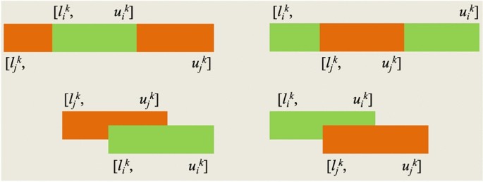

  

  Classification diagram of intersection operation for interval numbers.

• 2. Union operation

  $$ a_{k} (u_{i} ) \cup a_{k} (u_{j} ){ = }\left[ {\min (l_{i}^{k} ,l_{j}^{k} ),\max (u_{i}^{k} ,u_{j}^{k} )} \right] $$

  (2)

• 3. Complement operation

  $$ a_{k} (u_{i} )^{c} = \left( { - \infty ,l_{i}^{k} } \right) \cup \left( {u_{i}^{k} , + \infty } \right) $$

  (3)

• 4. Exclusion union operation

  $$ a_{k} (u_{i} ) \oplus a_{k} (u_{j} ) = \left\{ {\begin{array}{*{20}l} {\left\{ {a_{k}^{c} (u_{i} ) \cap a_{k}^{c} (u_{j} )} \right\}^{c} ,a_{k} (u_{i} ) \cap a_{k} (u_{j} ) = \emptyset } \hfill \\ {\left\{ {a_{k} (u_{i} ) \cup a_{k} (u_{j} )} \right\} \cap \left\{ {a_{k} (u_{i} ) \cup a_{k} (u_{j} )} \right\}^{c} ,{\text{ others}}} \hfill \\ \end{array} } \right. $$

  (4)

Distribution reduction based on an IIIS

Attribute reduction is a kind of knowledge reduction whose essence is to obtain the minimum attribute set. This section focuses on attribute reduction to solve the problems that there are too many attributes to be considered in the MADM process of low-carbon structural design for high-end equipment, which results in high complexity and large amount of decision-making computation. The minimum attribute set obtained contains low-carbon attributes which contributes to aiding in better green evaluation of high-end equipment structural schemes. According to different reduction rules, knowledge reduction can be divided into approximate reduction, distribution reduction, and maximum distribution reduction, among which the distribution coordination set is the core and foundation. Therefore, distribution reduction is adopted here to reduce redundant attributes of low-carbon structural design for high-end equipment.

In the actual decision-making process, expert evaluation for structural schemes on many attributes usually changes within a certain scope which are suitable to be described by interval numbers. At the same time, some expert evaluation may be incomplete due to the knowledge background restrictions and lack of technical means. Although it is difficult for experts to directly give the exact evaluation, they can quickly give the coarse-grained three-way opinions based on the structural schemes of similar products in history. For example, for a very reasonable structural scheme, experts give 'feasible' which is denoted by the numerical value 2. For an obviously unreasonable structural scheme, 'infeasible' is given with 0. If the structural scheme is not known well by experts, it obtains 'possible feasible' with 1. According to the coarse-grained three-way opinions provided by experts, the corresponding IIIS can be established³⁷.

Definition 1

³⁸Let K = (U, A_T ∪ D, V, F) be a decision-making system, where U called the domain is a finite set of objects denoted as{x₁, x₂, …, x_n}; A_T is a finite set of conditional attributes denoted as {a₁, a₂, …, a_m}; D = {d} is the set of finite target attributes; F is the set of relations between U and A_T which is represented as $F = \left\{ {f_{k} :U \to V_{k} ,k \le m} \right\}$; V_k is the finite range of a_k. If the conditional attribute value is expressed with interval numbers, for example, $f_{k} (x_{i} ,a_{k} ) = \left[ {l_{i}^{k} ,r_{i}^{k} } \right], \, l_{i}^{k} \le r_{i}^{k}$, and there exists x_i ∈ U, a_k ∈ A, f_k(x_i, a_k) = *, the decision-making system is called an IIIS where '*' means that the value in this position is incomplete.

A single-value decision-making system can conduct the classification directly based on the values of condition attributes, but its classification method is not applicable to the IIIS. Therefore, the improved incomplete interval similarity and the compatibility relation matrix are introduced to addressed this issue.

Definition 2

³⁹Suppose x_i and x_j ∈ U, and a_k ∈ A_T. When the attribute values of two objects x_i and x_j with respect to the attribute a_k are interval numbers no matter they are complete or incomplete, their similarity related to the attribute a_k is defined as follows.

$$ \alpha_{ij}^{k} { = }\left\{ {\begin{array}{*{20}l} {\frac{{\left| {\left[ {l_{i}^{k} ,r_{i}^{k} } \right] \cap \left[ {l_{j}^{k} ,r_{j}^{k} } \right]} \right|}}{{\left| {\left[ {l_{i}^{k} ,r_{i}^{k} } \right] \cup \left[ {l_{j}^{k} ,r_{j}^{k} } \right]} \right|}},f_{k} (x_{i} ,a_{k} ) = \left[ {l_{i}^{k} ,r_{i}^{k} } \right] \wedge f_{k} (x_{j} ,a_{k} ) = \left[ {l_{j}^{k} ,r_{j}^{k} } \right]} \hfill \\ {\frac{{\left[ {l_{i}^{k} ,r_{i}^{k} } \right]}}{{\left[ {\min V_{k} ,\max V_{k} } \right]}},f_{k} (x_{i} ,a_{k} ) = \left[ {l_{i}^{k} ,r_{i}^{k} } \right] \wedge f_{k} (x_{j} ,a_{k} ) = *} \hfill \\ {\frac{{\left[ {l_{j}^{k} ,r_{j}^{k} } \right]}}{{\left[ {\min V_{k} ,\max V_{k} } \right]}},f_{k} (x_{i} ,a_{k} ) = * \wedge f_{k} (x_{j} ,a_{k} ) = \left[ {l_{j}^{k} ,r_{j}^{k} } \right]} \hfill \\ {1,f_{k} (x_{i} ,a_{k} ) = * \wedge f_{k} (x_{j} ,a_{k} ) = *} \hfill \\ \end{array} } \right. $$

(5)

Definition 3

⁴⁰For the attribute a_k ∈ A_T, its α-compatibility relation matrix can be calculated as below:

$$ T_{{\left\{ {a_{k} } \right\}}}^{\alpha } = \left\{ {(u_{i} ,u_{j} ) \in U \times U\left| {\alpha_{ij}^{k} \ge \alpha } \right.} \right\} $$

(6)

where α is the similarity threshold which is artificially settled.

The α-compatibility relation matrix of the interval-valued decision-making system with respect to the set B ∈ A_T is defined as:

$$ T_{B}^{\alpha } = \left\{ {(u_{i} ,u_{j} ) \in U \times U\left| {\alpha_{ij}^{k} \ge \alpha ,a_{k} \in B} \right.} \right\} $$

(7)

If $T_{{\left\{ {a_{k} } \right\}}}^{\alpha }$ is the α-compatibility relation regarding the attribute a_k ∈ A_T, then the α-compatibility relation matrix is:

$$ T_{AT}^{\alpha } = \mathop \cap \limits_{{a_{k} \in AT}} T_{{\left\{ {a_{k} } \right\}}}^{\alpha } $$

(8)

For ease of expression, the α-compatibility relation matrix can be represented by the similarity rate Boolean matrix where the diagonal elements are 1 and all the elements are symmetric with respect to the diagonal.

Definition 4

³⁷Suppose B ∈ A_T and α ∈ [0, 1], the α-compatible class of the attribute set B is denoted as:

$$ S_{B}^{\alpha } \left( {u_{i} } \right) = \left\{ {u_{j} \in U;(u_{i} ,u_{j} ) \in T_{B}^{\alpha } } \right\} $$

(9)

The set of $S_{B}^{\alpha } \left( {u_{i} } \right)$ constitutes the coverage of the domain U, namely

$$ S_{B}^{\alpha } { = }\left\{ {S_{B}^{\alpha } \left( {u_{1} } \right),S_{B}^{\alpha } \left( {u_{2} } \right), \ldots ,S_{B}^{\alpha } \left( {u_{\left| U \right|} } \right)} \right\} $$

(10)

Definition 5

⁴¹Suppose $\forall B \in A_{T}$ and D_i ∈ U/IND({d}). For u_i ∈ U, the upper and lower rough approximations of decision-making attribute D = {d} with respect to the attribute set B are as follows.

$$ \overline{{Apr_{B}^{\alpha } }} (D) = \mathop \cup \limits_{i = 1}^{\left| U \right|} \left\{ {u_{i} \in U\left| {S_{B}^{\alpha } \left( {u_{i} } \right) \cap D_{i} \ne \emptyset } \right.} \right\} $$

(11)

$$ \underline{{Apr_{B}^{\alpha } }} (D) = \mathop \cup \limits_{i = 1}^{\left| U \right|} \left\{ {u_{i} \in U\left| {S_{B}^{\alpha } \left( {u_{i} } \right) \subseteq D_{i} } \right.} \right\} $$

(12)

Definition 6

⁴²If D_i ∈ U/IND(D) and B ∈ A_T, the approximate classification accuracy of the conditional attribute B is denoted as $\mu_{B}^{\alpha } (D)$.

$$ \mu_{B}^{\alpha } (D){ = }\frac{{\underline{{Apr_{B}^{\alpha } }} (D)}}{{\overline{{Apr_{B}^{\alpha } }} (D)}}{ = }\frac{{\left| {\mathop \cup \limits_{i = 1}^{\left| U \right|} \left\{ {u_{i} \in U\left| {S_{B}^{\alpha } \left( {u_{i} } \right) \subseteq D_{i} } \right.} \right\}} \right|}}{{\left| {\mathop \cup \limits_{i = 1}^{\left| U \right|} \left\{ {u_{i} \in U\left| {S_{B}^{\alpha } \left( {u_{i} } \right) \cap D_{i} \ne \emptyset } \right.} \right\}} \right|}} $$

(13)

Definition 7

⁴³If $B \in A_{T}$ when $x \in U$, it can be written as that U/IND(D) = {D₁, D₂, …, D_r}. Then the probability distribution of the IIIS is:

$$ \mu_{B}^{\alpha } (x){ = }\left( {\frac{{\left| {D_{1} \cap S_{B}^{\alpha } \left( x \right)} \right|}}{{\left| {S_{B}^{\alpha } \left( x \right)} \right|}},\frac{{\left| {D_{2} \cap S_{B}^{\alpha } \left( x \right)} \right|}}{{\left| {S_{B}^{\alpha } \left( x \right)} \right|}}, \cdots ,\frac{{\left| {D_{r} \cap S_{B}^{\alpha } \left( x \right)} \right|}}{{\left| {S_{B}^{\alpha } \left( x \right)} \right|}}} \right) $$

(14)

By the same token, $\mu_{A}^{\alpha } (x)$ and $r_{A} (x)$ can be calculated when B = A_T.

Definition 8

⁴³Suppose there is an IIIS denoted as K = (U, A, V, F) with B ∈ A_T and $\forall x \in U$ . If the attribute set B meets the following conditions:

• 1. $\mu_{B}^{\alpha } (x){ = }\mu_{AT}^{\alpha } (x)$;

• 2. There is no $C \subset B$ to meet the condition that $\mu_{C}^{\alpha } (x){ = }\mu_{AT}^{\alpha } (x)$;

Then the attribute subset B is called the distribution reduction of the IIIS based on the α-compatible class.

Specific operators of critical steps for low-carbon structural design

The minimum attribute set of low-carbon structural design

According to above distribution reduction principles in “Background knowledge” section, the minimum attribute set of low-carbon structural design for high-end equipment can be obtained as shown in Fig. 3. The related attributes in the minimum attribute set also can be divided into primary attributes and secondary attributes.

Figure 3

The minimum attribute set of low-carbon structural design for high-end equipment.

Causal effect judgment and weight calculation of decision-making attributes based on IRN-DANP

An important basis for the rational MADM of low-carbon structural design for high-end equipment is to accurately calculate attribute weights. However, the decision-making attributes in the minimum attribute set may not be independent of each other. As an extension of analytic hierarchy process (AHP), ANP can not only express the hierarchical relationship of these attributes but also reflect the interdependence among them, and then the causal effect which is very suitable for in-depth analysis of these attributes is available⁴⁴. DEMATEL can be used to modify the normalization operation of the super matrix in the original ANP model, forming DEMATEL-ANP, namely DANP⁴⁵. According to the risk preferences of experts, IRNs are good at dealing with uncertainties and can make decision results more in line with the actual situation. Therefore, IRN and DANP are combined to realize the causal effect analysis and attribute weight calculation of low-carbon structural design for high-end equipment under incomplete interval uncertainties.

Causal effect judgment of decision-making attributes for high-end equipment

The causal effect judgment of decision-making attributes for high-end equipment on low-carbon structural design is aimed at the internal factors of each group. The basic process is as follows.

• 1. Collect expert evaluation on attribute associations based on the minimum attribute set.

  Suppose there are m experts and the minimum attribute set of low-carbon structural design for high-end equipment contain n attributes. Each expert makes a judgment on the association between the attribute i and the attribute j by utilizing fuzzy languages which can be mapped to the integer number x_ij^k. The related mapping rules are shown in Table 1. Usually, it is difficult for experts to judge the degree of attribute association in the single point form. Therefore, their own cognition is often expressed in the form of an interval number denoted as $x_{ij}^{k} { = }\left[ {x_{ij}^{{k{ - }}} ,x_{ij}^{{k{ + }}} } \right]$.

  Table 1 Mapping rules between fuzzy languages of expert evaluation for attribute associations and integer numbers.

  The evaluation data of the expert k on attribute associations is represented by the square matrix X^k.

  $$ X^{k} = \left[ {\begin{array}{*{20}c} 0 & {[x_{12}^{k - } ,x_{12}^{k + } ]} & \cdots & {[x_{1n}^{k - } ,x_{1n}^{k + } ]} \\ {[x_{21}^{k - } ,x_{21}^{k + } ]} & 0 & \cdots & {[x_{2n}^{k - } ,x_{2n}^{k + } ]} \\ \vdots & \vdots & \ddots & \vdots \\ {[x_{n1}^{k - } ,x_{n1}^{k + } ]} & {[x_{n2}^{k - } ,x_{n2}^{k + } ]} & \cdots & 0 \\ \end{array} } \right] $$

  (15)

  where $x_{ij}^{k - }$ and $x_{ij}^{k + }$ are obtained through the language evaluation given by the expert k. k = 1, 2, …, m, and i = 1, 2, …, n.

  The evaluation matrices of all experts can be obtained in a similar way. The diagonal elements of each expert evaluation matrix are all 0, indicating that the attributes do not affect themselves. The left limit matrix X^k- and the right limit matrix X^k+ can be disassembled based on the expert evaluation matrix X^k.

  $$ X^{{k{ - }}} = \left[ {\begin{array}{*{20}c} 0 & {x_{12}^{k - } } & \cdots & {x_{1n}^{k - } } \\ {x_{21}^{k - } } & 0 & \cdots & {x_{2n}^{k - } } \\ \vdots & \vdots & \ddots & \vdots \\ {x_{n1}^{k - } } & {x_{n2}^{k - } } & \cdots & 0 \\ \end{array} } \right] $$

  (16)
  $$ X^{{k{ + }}} = \left[ {\begin{array}{*{20}c} 0 & {x_{12}^{k + } } & \cdots & {x_{1n}^{k + } } \\ {x_{21}^{k + } } & 0 & \cdots & {x_{2n}^{k + } } \\ \vdots & \vdots & \ddots & \vdots \\ {x_{n1}^{k + } } & {x_{n2}^{k + } } & \cdots & 0 \\ \end{array} } \right] $$

  (17)

  Since the expert k may not have a comprehensive understanding of all attributes, it may be difficult to give all the values of X^k and the incomplete data are represented by *. Reasonable completion of these incomplete interval data is very important for the subsequent calculation.

• 2. Complete the incomplete interval evaluation data with a collaborative filtering algorithm based on expert consensus.

  MADM with incomplete data is common in the structural design for high-end equipment, and there are two main solutions for this issue. The former is to delete the structural schemes of high-end equipment which contain vacant values, and then make decisions using the remaining data. However, it inevitably wastes some existing data. The latter is to complete the incomplete data and then make decisions based on the completed data. It can make full use of the existing data and largely eliminate the impact of incomplete data on decision-making results. Since all experts have certain professional knowledge background and work experience, even though some experts' decision-making data may be different, all experts' decision-making data may not be completely contrary to each other, and there should be still a high degree of similarity which can be called expert consensus. Therefore, a collaborative filtering algorithm denoted expert consensus is adopted for data completion in the MADM process of low-carbon structural design⁴⁶. In view of the mature development of collaborative filtering algorithms, this section does not elaborate it further to save space.

• 3. Calculate the interval rough average incidence matrix of decision-making attributes based on completed evaluation.

  According to X¹, X², …, and X^m, two average incidence matrices can be obtained as follows:

  $$ X^{* - } = \left[ {\begin{array}{*{20}c} {x_{11}^{1 - } ,x_{11}^{2 - } , \cdots x_{11}^{m - } } & {x_{12}^{1 - } ,x_{12}^{2 - } , \cdots x_{12}^{m - } } & \cdots & {x_{1n}^{1 - } ,x_{1n}^{2 - } , \cdots x_{1n}^{m - } } \\ {x_{21}^{1 - } ,x_{21}^{2 - } , \cdots x_{21}^{m - } } & {x_{22}^{1 - } ,x_{22}^{2 - } , \cdots x_{22}^{m - } } & \cdots & {x_{2n}^{1 - } ,x_{2n}^{2 - } , \cdots x_{2n}^{m - } } \\ \vdots & \vdots & \ddots & \vdots \\ {x_{n1}^{1 - } ,x_{n1}^{2 - } , \cdots x_{n1}^{m - } } & {x_{n2}^{1 - } ,x_{n2}^{2 - } , \cdots x_{n2}^{m - } } & \cdots & {x_{nn}^{1 - } ,x_{nn}^{2 - } , \cdots x_{nn}^{m - } } \\ \end{array} } \right] $$

  (18)
  $$ X^{* + } = \left[ {\begin{array}{*{20}c} {x_{11}^{1 + } ,x_{11}^{2 + } , \cdots x_{11}^{m + } } & {x_{12}^{1 + } ,x_{12}^{2 + } , \cdots x_{12}^{m + } } & \cdots & {x_{1n}^{1 + } ,x_{1n}^{2 + } , \cdots x_{1n}^{m + } } \\ {x_{21}^{1 + } ,x_{21}^{2 + } , \cdots x_{21}^{m + } } & {x_{22}^{1 + } ,x_{22}^{2 + } , \cdots x_{22}^{m + } } & \cdots & {x_{2n}^{1 + } ,x_{2n}^{2 + } , \cdots x_{2n}^{m + } } \\ \vdots & \vdots & \ddots & \vdots \\ {x_{n1}^{1 + } ,x_{n1}^{2 + } , \cdots x_{n1}^{m + } } & {x_{n2}^{1 + } ,x_{n2}^{2 + } , \cdots x_{n2}^{m - } } & \cdots & {x_{nn}^{1 + } ,x_{nn}^{2 + } , \cdots x_{nn}^{m + } } \\ \end{array} } \right] $$

  (19)

  where $x_{ij}^{k - }$ and $x_{ij}^{k + }$ are transformed into the interval approximations, namely

  $$ IRN(x_{ij}^{k} ) = \left[ {RN(x_{ij}^{k - } ),RN(x_{ij}^{{k{ + }}} )} \right] $$

  (20)
  $$ RN(x_{ij}^{k - } ){ = }\left[ {\underline{Lim} (x_{ij}^{k - } ),\overline{Lim} (x_{ij}^{k - } )} \right] $$

  (21)
  $$ RN(x_{ij}^{{k{ + }}} ) = \left[ {\underline{Lim} (x_{ij}^{{k{ + }}} ),\overline{Lim} (x_{ij}^{{k{ + }}} )} \right] $$

  (22)
  $$ IRN(x_{ij}^{k} ) = \left\{ {\left[ {\underline{Lim} (x_{ij}^{k - } ),\overline{Lim} (x_{ij}^{k - } )} \right],\left[ {\underline{Lim} (x_{ij}^{{k{ + }}} ),\overline{Lim} (x_{ij}^{{k{ + }}} )} \right]} \right\} $$

  (23)

  where $\underline{Lim} (x_{ij}^{k - } )$ and $\underline{Lim} (x_{ij}^{{k{ + }}} )$ represent the lower limits of $RN(x_{ij}^{k - } )$ and $RN(x_{ij}^{{k{ + }}} )$, and $\overline{Lim} (x_{ij}^{k - } )$ and $\overline{Lim} (x_{ij}^{{k{ + }}} )$ represent the upper limits of $RN(x_{ij}^{k - } )$ and $RN(x_{ij}^{{k{ + }}} )$.

  According to the influence degree of the attribute i on the attribute j, an interval approximation including all expert evaluation can be obtained.

  $$ RN(x_{ij}^{ - } ){ = }\left\{ {\left[ {\underline{Lim} (x_{ij}^{1 - } ),\overline{Lim} (x_{ij}^{1 - } )} \right],\left[ {\underline{Lim} (x_{ij}^{2 - } ),\overline{Lim} (x_{ij}^{2 - } )} \right], \ldots ,\left[ {\underline{Lim} (x_{ij}^{m - } ),\overline{Lim} (x_{ij}^{m - } )} \right]} \right\} $$

  (24)
  $$ RN(x_{ij}^{ + } ){ = }\left\{ {\left[ {\underline{Lim} (x_{ij}^{1 + } ),\overline{Lim} (x_{ij}^{1 + } )} \right],\left[ {\underline{Lim} (x_{ij}^{2 + } ),\overline{Lim} (x_{ij}^{2 + } )} \right], \ldots ,\left[ {\underline{Lim} (x_{ij}^{m + } ),\overline{Lim} (x_{ij}^{m + } )} \right]} \right\} $$

  (25)

  The average approximate interval including all expert evaluation is as below.

  $$ RN(z_{ij}^{ - } ){ = }\left[ {\underline{Lim} (z_{ij}^{ - } ),\overline{Lim} (z_{ij}^{ - } )} \right] = \left\{ {\begin{array}{*{20}c} {\underline{Lim} (z_{ij}^{ - } ) = \frac{1}{m}\sum\limits_{k = 1}^{m} {\underline{Lim} (x_{ij}^{k - } )} } \\ {\overline{Lim} (z_{ij}^{ - } ) = \frac{1}{m}\sum\limits_{k = 1}^{m} {\overline{Lim} (x_{ij}^{k - } )} } \\ \end{array} } \right. $$

  (26)
  $$ RN(z_{ij}^{ + } ){ = }\left[ {\underline{Lim} (z_{ij}^{ + } ),\overline{Lim} (z_{ij}^{ + } )} \right] = \left\{ {\begin{array}{*{20}c} {\underline{Lim} (z_{ij}^{ + } ) = \frac{1}{m}\sum\limits_{k = 1}^{m} {\underline{Lim} (x_{ij}^{{k{ + }}} )} } \\ {\overline{Lim} (z_{ij}^{ + } ) = \frac{1}{m}\sum\limits_{k = 1}^{m} {\overline{Lim} (x_{ij}^{{k{ + }}} )} } \\ \end{array} } \right. $$

  (27)

  where $IRN(z_{ij} ){ = }\left[ {RN(z_{ij}^{ - } ),RN(z_{ij}^{ + } )} \right]$.

  The interval rough average incidence matrix Z of decision-making attributes for low-carbon structural design in IRNs can be obtained.

  $$ Z = \left[ {\begin{array}{*{20}c} 0 & {IRN(z_{12} )} & \cdots & {IRN(z_{1n} )} \\ {IRN(z_{21} )} & 0 & \cdots & {IRN(z_{2n} )} \\ \vdots & \vdots & \ddots & \vdots \\ {IRN(z_{n1} )} & {IRN(z_{n2} )} & \cdots & 0 \\ \end{array} } \right] $$

  (28)

  The matrix Z represents the interactions between different attributes of structural schemes. The sum of the elements in the ith row of Z represents the combined influence which the attribute i has on other attributes, and the sum of the elements in the jth column represents the combined influence which other attributes have on the attribute j.

• 4. Calculate the initial direct correlation matrix of decision-making attributes.

  The initial direct correlation matrix of decision-making attributes, denoted as $D = \left[ {IRN(d_{ij} )} \right]_{n \times n}$, can be obtained.

  $$ D = \left[ {\begin{array}{*{20}c} 0 & {IRN(d_{12} )} & \cdots & {IRN(d_{1n} )} \\ {IRN(d_{21} )} & 0 & \cdots & {IRN(d_{2n} )} \\ \vdots & \vdots & \ddots & \vdots \\ {IRN(d_{n1} )} & {IRN(d_{n2} )} & \cdots & 0 \\ \end{array} } \right] $$

  (29)

  where IRN (d_ij) is as below.

  $$ IRN(d_{ij} ){ = }\frac{{IRN(z_{ij} )}}{IRN(s)}{ = }IRN\left( {\left[ {\frac{{z_{ij}^{ - } }}{{s_{ij}^{ - } }},\frac{{z_{ij}^{ + } }}{{s_{ij}^{ + } }}} \right],\left[ {\frac{{z_{ij}^{^{\prime} - } }}{{s_{ij}^{^{\prime} - } }},\frac{{z_{ij}^{^{\prime} + } }}{{s_{ij}^{^{\prime} + } }}} \right]} \right) $$

  (30)

  The IRN(s) can be obtained by Formulas (26) and (27).

  $$ IRN(s) = \left( {\left[ {\max (\sum\limits_{j = 1}^{n} {z_{ij}^{ - } } ),\max (\sum\limits_{j = 1}^{n} {z_{ij}^{ + } } )} \right],\left[ {\max (\sum\limits_{j = 1}^{n} {z_{ij}^{{^{\prime} - }} } ),\max (\sum\limits_{j = 1}^{n} {z_{ij}^{{^{\prime} + }} } )} \right]} \right) $$

  (31)

  where $IRN(d_{ij} ) = \left[ {RN(d_{ij}^{ - } ),RN(d_{ij}^{ + } )} \right]$ represents the direct influence which the attribute i has on the attribute j.

• 5. Calculate the global incidence matrix of decision-making attributes.

  Since each IRN has an upper approximation and an lower approximation, the initial direct incidence matrix $D = \left[ {IRN\left( {d_{ij} } \right)} \right]_{n \times n}$ can be decomposed into four submatrices, namely $D = \left( {\left[ {D^{ - } ,D^{ + } } \right],\left[ {D^{\prime - } ,D^{\prime + } } \right]} \right)$, where $D^{ - } = \left[ {\underline{Lim} \left( {d_{ij} } \right)} \right]_{n \times n}$, $D^{ + } = \left[ {\overline{Lim} \left( {d_{ij} } \right)} \right]_{n \times n}$, $D^{\prime - } = \left[ {\underline{Lim} \left( {d^{\prime}_{ij} } \right)} \right]_{n \times n}$, and $D^{ \prime+ } = \left[ {\overline{Lim} \left( {d^{\prime}_{ij} } \right)} \right]_{n \times n}$. Let O represent the zero matrix in the nth order, then $\mathop {\lim }\limits_{m \to \infty } (D^{ - } )^{m} = \mathop {\lim }\limits_{m \to \infty } (D^{ + } )^{m} = \mathop {\lim }\limits_{m \to \infty } (D^{^{\prime} - } )^{m} = \mathop {\lim }\limits_{m \to \infty } (D{\prime}^{ + } )^{m} = O$.

  $$ \left\{ \begin{gathered} \mathop {\lim }\limits_{m \to \infty } \left[ {1{ + }D^{ - } { + (}D^{ - } {)}^{2} + \cdots + {(}D^{ - } {)}^{m} } \right] = [1 - D^{ - } ]^{ - 1} \hfill \\ \vdots \hfill \\ \mathop {\lim }\limits_{m \to \infty } \left[ {1{ + }D^{^{\prime} + } { + (}D^{^{\prime} + } {)}^{2} + \cdots + {(}D^{^{\prime} + } {)}^{m} } \right] = [1 - D^{^{\prime} + } ]^{ - 1} \hfill \\ \end{gathered} \right. $$

  (32)

  where I represents the identity matrix in the nth order.

  For the interval rough global incidence matrix $T = \left[ {IRN(t_{ij} )} \right]_{n \times n}$, $IRN(t_{ij} ) = \left[ {RN(t_{ij}^{ - } ),RN(t_{ij}^{ + } )} \right]$ represents the indirect influence exerted by the attribute i on the attribute j. The matrix T represents the mutual influence between different attributes. According to the same idea, the matrix T is divided into four submatrices, namely T = ([T^-, T⁺], [T^’-, T^’+]).

• 6. Calculate the sums of row elements and column elements in the global incidence matrix.

  The sums of row elements and column elements of the matrix T are represented by R and C, respectively.

  $$ IRN(R_{i} ) = \left[ {\sum\limits_{j = 1}^{n} {IRN(t_{ij} )} } \right]_{n \times 1} = \left[ {\left( {\left[ {\sum\limits_{j = 1}^{n} {t_{ij}^{ - } } ,\sum\limits_{j = 1}^{n} {t_{ij}^{ + } } } \right],\left[ {\sum\limits_{j = 1}^{n} {t_{ij}^{^{\prime} - } } ,\sum\limits_{j = 1}^{n} {t_{ij}^{^{\prime} + } } } \right]} \right)} \right]_{n \times 1} $$

  (33)
  $$ IRN(C_{i} ) = \left[ {\sum\limits_{i = 1}^{n} {IRN(t_{ij} )} } \right]_{n \times 1} = \left[ {\left( {\left[ {\sum\limits_{i = 1}^{n} {t_{ij}^{ - } } ,\sum\limits_{i = 1}^{n} {t_{ij}^{ + } } } \right],\left[ {\sum\limits_{i = 1}^{n} {t_{ij}^{^{\prime} - } } ,\sum\limits_{i = 1}^{n} {t_{ij}^{^{\prime} + } } } \right]} \right)} \right]_{n \times 1} $$

  (34)

  where R_i denotes the sum of all elements in the ith row of the matrix T, representing the overall influence which the attribute i transmits to other attributes. C_i denotes the sum of all elements of the ith column of the matrix T, representing the overall influence which the attribute i receives from the other attributes. When i = j, (R_i + C_i) represents the influence degree of the attribute i, and (R_i-C_i) represents the influence density of the attribute i related to other attributes.

• 7. Set the causality threshold of decision-making attributes and draw the related causal effect diagrams.

  Based on the global incidence matrix T, the causality threshold of decision-making attributes denoted as α is set to be the average value of its elements, and the causal effect diagrams can be obtained.

  $$ \alpha { = }\frac{{\sum\limits_{i = 1}^{n} {\sum\limits_{j = 1}^{n} {IRN(t_{ij} )} } }}{N} $$

  (35)

  where N represents the total number of elements contained in the matrix T.

  The complex relationships between decision-making attributes can be visualized by causal effect diagrams. Important attributes can be selected and how these important attributes affect other attributes can be identified. The elements in the matrix T which are larger than the threshold are selected to get the causal effect diagrams. The x-axis represents IRN(R_i + C_i), and the y-axis represents IRN(R_i-C_i). The directed arrows of causality start from the attributes with values below the threshold α and point to the attributes with values above the threshold α. Weights of decision-making attributes are obtained when the causal relationships between attributes are clarified.

Weight calculation of decision-making attributes

Weight calculation of decision-making attributes for low-carbon structural design are available as follows.

• 1. Obtain the global incidence matrix of decision-making attributes for low-carbon structural design in IRNs.

  The global incidence matrix of primary attributes, denoted as T_D, is obtained according to Sect. “Causal effect judgment of decision-making attributes for high-end equipment”.

  $$ T_{D} = \left[ {\begin{array}{*{20}c} {t_{D}^{11} } & {t_{D}^{12} } & \cdots & {t_{D}^{1n} } \\ {t_{D}^{21} } & {t_{D}^{22} } & \cdots & {t_{D}^{2n} } \\ \vdots & \vdots & \ddots & \vdots \\ {t_{D}^{n1} } & {t_{D}^{n2} } & \cdots & {t_{D}^{nn} } \\ \end{array} } \right] $$

  (36)

  where $t_{D}^{ij}$ represents the influence which the primary attribute D_i has on the primary attribute D_j, and i, j = 1, 2, …, n. If i = j, $t_{D}^{ij} = 0$.

  $IRN(t_{{c_{{ik_{1} }} }}^{{c_{{jk_{2} }} }} )$ denotes the influence which the secondary attributes $c_{{ik_{1} }}$ in the primary attribute D_i has on the secondary attribute $c_{{jk_{2} }}$ in the primary attribute D_j, where $i,j = 1,2, \cdots ,n$, k₁ = 1, 2, …, n_i, and k₂ = 1, 2, …, n_j. n_i and n_j represent the numbers of the secondary attributes in primary attributes D_i and D_j, respectively.

  $$ T_{C}^{ij} = \left[ {\begin{array}{*{20}c} {IRN\left( {t_{{c_{i1} }}^{{c_{j1} }} } \right)} & {IRN\left( {t_{{c_{i1} }}^{{c_{j2} }} } \right)} & \cdots & {IRN\left( {t_{{c_{i1} }}^{{c_{{jn_{j} }} }} } \right)} \\ {IRN\left( {t_{{c_{i2} }}^{{c_{j1} }} } \right)} & {IRN\left( {t_{{c_{i2} }}^{{c_{j2} }} } \right)} & \cdots & {IRN\left( {t_{{c_{i2} }}^{{c_{{jn_{j} }} }} } \right)} \\ \vdots & \vdots & \ddots & \vdots \\ {IRN\left( {t_{{c_{{in_{i} }} }}^{{c_{j1} }} } \right)} & {IRN\left( {t_{{c_{{in_{i} }} }}^{{c_{j2} }} } \right)} & \cdots & {IRN\left( {t_{{c_{{in_{i} }} }}^{{c_{{jn_{j} }} }} } \right)} \\ \end{array} } \right] $$

  (37)

  Then, the global incidence matrix for the secondary attributes is obtained, which is denoted as T_C.

  

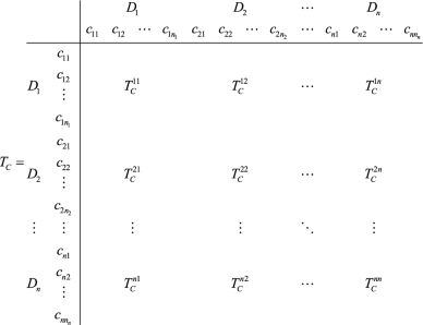  (38)

  It is necessary to use the mathematical operations of IRNs to standardize the global incidence matrix T_D, T_C, and $T_{C}^{ij}$⁴⁷. Let IRN(A) = ([A₁, A₂], [A₃, A₄]) and IRN(B) = ([B₁, B₂], [B₃, B₄]).

  $$ IRN\left( A \right) \, + IRN\left( B \right) \, = \, \left( {\left[ {A_{{1}} + B_{{1}} ,A_{{2}} + B_{{2}} } \right], \, \left[ {A_{{3}} + B_{{3}} ,A_{{4}} + B_{{4}} } \right]} \right) $$

  (39)
  $$ IRN\left( A \right) \, - IRN\left( B \right) \, = \, \left( {\left[ {A_{{1}} - B_{{1}} ,A_{{2}} - B_{{2}} } \right], \, \left[ {A_{{3}} - B_{{3}} ,A_{{4}} - B_{{4}} } \right]} \right) $$

  (40)
  $$ IRN\left( A \right) \times IRN\left( B \right) \, = \, ([A_{{1}} \times B_{{1}} ,A_{{2}} \times B_{{2}} ],[A_{{3}} \times B_{{3}} ,A_{{4}} \times B_{{4}} ]) $$

  (41)
  $$ IRN\left( A \right)/IRN\left( B \right) \, = \, ([A_{{1}} /B_{{4}} ,A_{{2}} /B_{{3}} \left] {, \, } \right[A_{{3}} /B_{{2}} ,A_{{4}} /B_{{1}} ]) $$

  (42)
  $$ k \times IRN\left( A \right) \, = \, ([k \times A_{{1}} ,k \times A_{{2}} ],[k \times A_{{3}} ,k \times A_{{4}} ]) $$

  (43)

  Let T_D, T_C, and $T_{C}^{ij}$ be transformed into T_D#, T_C#, and $T_{{C{{\# }}}}^{ij}$ after the standardization operation, respectively.

  $$ T_{{D{{\# }}}} = \left[ {\begin{array}{*{20}c} {IRN(t_{D\# }^{11} )} & {IRN(t_{D\# }^{12} )} & \cdots & {IRN(t_{Q\# }^{1n} )} \\ {IRN(t_{D\# }^{21} )} & {IRN(t_{D\# }^{22} )} & \cdots & {IRN(t_{D\# }^{2n} )} \\ \vdots & \vdots & \vdots & \vdots \\ {IRN(t_{D\# }^{n1} )} & {IRN(t_{D\# }^{n2} )} & \cdots & {IRN(t_{D\# }^{nn} )} \\ \end{array} } \right] $$

  (44)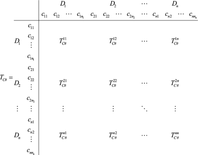
  

  (45)

  Set the standardized matrix of the interval rough matrix T_q as T_q#.

  $$ T_{Q} = \left[ {\begin{array}{*{20}c} {IRN(t_{Q}^{11} )} & {IRN(t_{Q}^{12} )} & \cdots & {IRN(t_{Q}^{1l} )} \\ {IRN(t_{Q}^{21} )} & {IRN(t_{Q}^{22} )} & \cdots & {IRN(t_{Q}^{2l} )} \\ \vdots & \vdots & \ddots & \vdots \\ {IRN(t_{Q}^{h1} )} & {IRN(t_{Q}^{h2} )} & \cdots & {IRN(t_{Q}^{hl} )} \\ \end{array} } \right] $$

  (46)
  $$ T_{{Q{{\# }}}} { = }\left[ {\begin{array}{*{20}c} {IRN(t_{Q\# }^{11} )} & {IRN(t_{Q\# }^{12} )} & \cdots & {IRN(t_{Q\# }^{1l} )} \\ {IRN(t_{Q\# }^{21} )} & {IRN(t_{Q\# }^{22} )} & \cdots & {IRN(t_{Q\# }^{2l} )} \\ \vdots & \vdots & \ddots & \vdots \\ {IRN(t_{Q\# }^{h1} )} & {IRN(t_{Q\# }^{h2} )} & \cdots & {IRN(t_{Q\# }^{hl} )} \\ \end{array} } \right]{ = }\left[ {\begin{array}{*{20}c} {\frac{{IRN(t_{Q}^{11} )}}{{IRN(d_{1} )}}} & {\frac{{IRN(t_{Q}^{12} )}}{{IRN(d_{1} )}}} & \cdots & {\frac{{IRN(t_{Q}^{1l} )}}{{IRN(d_{1} )}}} \\ {\frac{{IRN(t_{Q}^{21} )}}{{IRN(d_{2} )}}} & {\frac{{IRN(t_{Q}^{22} )}}{{IRN(d_{2} )}}} & \cdots & {\frac{{IRN(t_{Q}^{2l} )}}{{IRN(d_{2} )}}} \\ \vdots & \vdots & \ddots & \vdots \\ {\frac{{IRN(t_{Q}^{h1} )}}{{IRN(d_{h} )}}} & {\frac{{IRN(t_{Q}^{h2} )}}{{IRN(d_{h} )}}} & \cdots & {\frac{{IRN(t_{Q}^{hl} )}}{{IRN(d_{h} )}}} \\ \end{array} } \right] $$

  (47)

  where IRN(d_f) represents the sum of the interval rough elements in the fth row of the matrix T_q, and f = 1, 2, …, h.

  $$ IRN(d_{f} ) = \sum\limits_{g = 1}^{l} {IRN(t_{Q}^{fg} } ) $$

  (48)

• 2. Establish the unweighted hypermatrix of decision-making attributes.

  Since the global incidence matrix T_C indicates the mutual influence between different attributes, the normalized global incidence matrix T_C# can be transposed based on ANP to obtain the unweighted hypermatrix represented as W = [T_C#]^T.

  

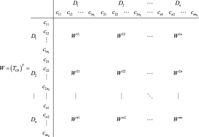  (49)

  where $W^{11} = \left( {T_{C\# }^{11} } \right)^{T}$, and other values of W^ij can be obtained in this way.

• 3. Establish the weighted standard hypermatrix of decision-making attributes.

  The elements in the weighted standard hypermatrix W_q are obtained by multiplying the elements in the unweighted hypermatrix W with the elements in the standardized global incidence matrix T_D#.

  

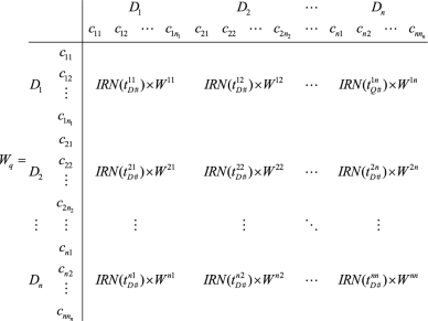  (50)

• 4. Output the interval rough weights of decision-making attributes.

  If the weighted standard hypermatrix W_q is multiplied by itself for a certain number of times, it will become a limit super matrix in a long-term stable state which is denoted as $W_{q}^{J}$ in interval rough numbers. The global priority vector of $W_{q}^{J}$ is the weight distribution vector of decision-making attributes in IRNs, and then each attribute weight can be obtained as follows.

  $$ \mathop {\lim }\limits_{k \to \infty } = \left( {W_{q} } \right)^{k} = W_{q}^{J} $$

  (51)

Ranking of alternative low-carbon structural schemes for high-end equipment based on IRN-MABAC

The subsequent MADM process and its ranking results of alternative low-carbon structural schemes for high-end equipment can be available after analyzing the cause-effect relationships and attribute weights. Compared with well-known decision-making tools such as VIKOR and TOPSIS, MABAC can rank the advantages and disadvantages of each alternative only according to its boundary approximation region, which is very conducive to obtaining accurate decision-making results under uncertain conditions^48,49. In this section, MABAC and IRN are combined to obtain the advantages and disadvantages of alternative low-carbon structural schemes and determine which is the best.

Approximation regions of attribute boundary for alternative low-carbon structural schemes

According to the basic idea of MABAC, m experts on the targeted high-end equipment are invited to give professional evaluation on b alternative low-carbon structural schemes (denoted as a₁, a₂, …, a_b) under n decision-making attributes. Each expert makes a judgment on the performance of a_i under the decision-making attribute c_j, where '1' means extremely bad, '2' means very bad, '3' means bad, '4' means ordinary, '5' means good, '6' means very good, and '7' means extremely good. The minimum attribute set of low-carbon structural design for high-end equipment shown in Fig. 3 is refined to secondary attributes, the alternative structural schemes are directly evaluated under secondary attributes. Let the expert k express his/her performance evaluation for a_i under c_j in the form of interval numbers, which is denoted as u_ij^k = [u_ij^k-, u_ij^k+], where k = 1, 2, …, m. A collaborative filtering algorithm mentioned is used to addressed the incomplete expert evaluation⁴⁴. By synthesizing the evaluation data of m experts, the interval rough average decision-making matrix U of alternative low-carbon structural schemes can be obtained.

(52)

where IRN (u_ij) is the interval rough evaluation of the alternative low-carbon structural scheme a_i under the decision-making attribute c_j, and

$$ IRN(u_{ij} ){ = }\left[ {RN(u_{ij}^{ - } ),RN(u_{ij}^{ + } )} \right] = \left\{ {\left[ {\underline{Lim} (u_{ij}^{ - } ),\overline{Lim} (u_{ij}^{ - } )} \right],\left[ {\underline{Lim} (u_{ij}^{ + } ),\overline{Lim} (u_{ij}^{ + } )} \right]} \right\} $$

(53)

The decision-making attributes of low-carbon structural schemes for high-end equipment are divided into positive attributes and negative attributes. For positive attributes such as quality stability and fatigue life, the higher the evaluation value, the better the high-end equipment structural scheme. For negative attributes such as economic cost and running noise, the lower the evaluation value, the better the high-end equipment structural scheme.

The standard average decision-making matrix of structural schemes is denoted as U^S in IRNs.

(54)

$P_{i}^{ - }$ and $P_{i}^{ + }$ represent the minimum values of the lower limit and the upper limit of the interval approximation for all alternative structural schemes under the observed attribute, respectively.

$$ P_{i}^{ - } = \mathop {\min }\limits_{i} \left\{ {\underline{Lim} (u_{ij}^{ - } ),\underline{Lim} (u_{ij}^{ + } )} \right\} $$

(55)

$$ P_{i}^{ + } = \mathop {\min }\limits_{i} \left\{ {\overline{Lim} (u_{ij}^{ - } ),\overline{Lim} (u_{ij}^{ + } )} \right\} $$

(56)

For positive attributes,

$$ IRN(u_{ij}^{s} ) = \left\{ {\left[ {\frac{{\underline{Lim} (u_{ij}^{ - } ) - P_{i}^{ - } }}{{P_{i}^{ + } - P_{i}^{ - } }},\frac{{\overline{Lim} (u_{ij}^{ - } ) - P_{i}^{ - } }}{{P_{i}^{ + } - P_{i}^{ - } }}} \right],\left[ {\frac{{\underline{Lim} (u_{ij}^{ + } ) - P_{i}^{ - } }}{{P_{i}^{ + } - P_{i}^{ - } }},\frac{{\overline{Lim} (u_{ij}^{ + } ) - P_{i}^{ - } }}{{P_{i}^{ + } - P_{i}^{ - } }}} \right]} \right\} $$

(57)

For negative attributes,

$$ IRN(u_{ij}^{s} ) = \left\{ {\left[ {\frac{{\overline{Lim} (u_{ij}^{ + } ) - P_{i}^{ + } }}{{P_{i}^{ - } - P_{i}^{ + } }},\frac{{\underline{Lim} (u_{ij}^{ + } ) - P_{i}^{ + } }}{{P_{i}^{ - } - P_{i}^{ + } }}} \right],\left[ {\frac{{\overline{Lim} (u_{ij}^{ - } ) - P_{i}^{ + } }}{{P_{i}^{ + } - P_{i}^{ - } }},\frac{{\underline{Lim} (u_{ij}^{ + } ) - P_{i}^{ + } }}{{P_{i}^{ + } - P_{i}^{ - } }}} \right]} \right\} $$

(58)

The interval rough weighted decision-making matrix of structural schemes is denoted as WU^S.

(59)

IRN(w_j) is the interval rough weight of the decision-making attribute c_j, then:

$$ IRN(wu_{ij}^{s} ) = IRN(w_{j} ) \times IRN(u_{ij}^{s} ) + IRN(w_{j} ) $$

(60)

where i = 1, 2, …, b. b is the total number of alternative structural schemes. j = 1, 2, …, n, and n is the total number of secondary attributes.

Let the boundary approximation region matrix of alternative structural schemes with the specification of 1 × n be represented by B.

(61)

where the element IRN (b_j) represents the boundary approximation region of the decision-making attribute c_j, and

$$ IRN(b_{j} ) = \left[ {\mathop \Pi \limits_{i = 1}^{l} IRN(wu_{ij}^{s} )} \right]^{\frac{1}{l}} = \left\{ {\left[ {\left( {\mathop \Pi \limits_{i = 1}^{l} IRN\underline{Lim} (u_{ij}^{ - } )} \right)^{\frac{1}{l}} ,\left( {\mathop \Pi \limits_{i = 1}^{l} IRN\overline{Lim} (u_{ij}^{ - } )} \right)^{\frac{1}{l}} } \right],\left[ {\left( {\mathop \Pi \limits_{i = 1}^{l} IRN\underline{Lim} (u_{ij}^{ + } )} \right)^{\frac{1}{l}} ,\left( {\mathop \Pi \limits_{i = 1}^{l} IRN\overline{Lim} (u_{ij}^{ + } )} \right)^{\frac{1}{l}} } \right]} \right\} $$

(62)

Ranking strategies of alternative low-carbon structural schemes

The distance matrix of alternative low-carbon structural schemes is represented by J = [IRN(J_ij)]_b×n, where the element IRN(J_ij) represents the distance between the structural scheme a_i and the boundary approximation region of the decision-making attribute c_j. This distance is the difference between the element $IRN(wu_{ij}^{s} )$ in the weighted decision-making matrix WU^S and the element IRN (b_j) in the boundary approximation region matrix B for alternative structural schemes.

$$ J{ = }\left[ {\begin{array}{*{20}c} {IRN(wu_{11}^{s} )} & {IRN(wu_{12}^{s} )} & \cdots & {IRN(wu_{1n}^{s} )} \\ {IRN(wu_{21}^{s} )} & {IRN(wu_{22}^{s} )} & \cdots & {IRN(wu_{2n}^{s} )} \\ \vdots & \vdots & \ddots & \vdots \\ {IRN(wu_{b1}^{s} )} & {IRN(wu_{b2}^{s} )} & \cdots & {IRN(wu_{bn}^{s} )} \\ \end{array} } \right]{ - }\left[ {\begin{array}{*{20}c} {IRN(b_{1} )} & {IRN(b_{2} )} & \cdots & {IRN(b_{n} )} \\ {IRN(b_{1} )} & {IRN(b_{2} )} & \cdots & {IRN(b_{n} )} \\ \vdots & \vdots & \ddots & \vdots \\ {IRN(b_{1} )} & {IRN(b_{2} )} & \cdots & {IRN(b_{n} )} \\ \end{array} } \right] $$

(63)

where i = 1, 2, …, b. b is the total number of alternative low-carbon structural schemes. j = 1, 2, …, n, and n is the total number of secondary attributes.

If IRN (J_ij) > IRN (b_j), the alternative low-carbon structural scheme a_i is closer to the positive ideal structural scheme under the decision-making attribute c_j. If IRN (J_ij) < IRN (b_j), the alternative low-carbon structural scheme a_i is closer to the negative ideal structural scheme under the decision-making attribute c_j. However, there are multiple attributes should be considered in the MADM process of low-carbon structural design for high-end equipment. The best low-carbon structural scheme needs to be as close as possible to the positive ideal structural scheme under all decision-making attributes.

Let the sum of the elements in the ith row of the distance matrix J be represented by IRN(J_i), which is the synthesis distance of the boundary approximation regions of the alternative low-carbon structural scheme a_i for all decision-making attributes. The larger its value is, the more ideal the alternative low-carbon structural scheme is.

$$ IRN(J_{i} ) = \sum\limits_{j = 1}^{n} {IRN(J_{ij} )} $$

(64)

IRN(A) is set as $IRN(A){ = [}RN(A^{ - } ),RN(A^{ + } )] = \{ [\underline{Lim} (A^{ - } ),\overline{Lim} (A^{ - } ){],[}\underline{Lim} (A^{ + } ),\overline{Lim} (A^{ + } )]\}$, and JD(A) is the related interval rough joint point.

$$ JD(A) = \mu_{A} \cdot \underline{Lim} (A^{ - } ) + (1 - \mu_{A} )\overline{Lim} (A^{ + } ) $$

(65)

where $\mu_{A}$ is its interval rough ratio, and

$$ \mu_{A} { = }\frac{{\overline{Lim} (A^{ + } ){ - }\underline{Lim} (A^{ + } )}}{{[\overline{Lim} (A^{ + } ){ - }\underline{Lim} (A^{ + } )] + [\overline{Lim} (A^{ - } ){ - }\underline{Lim} (A^{ - } )]}} $$

(66)

The interval rough synthesis distances of the alternative low-carbon structural scheme a_p and the alternative low-carbon structural scheme a_q to the boundary approximation region of all attributes are represented as IRN(p) and IRN(q), respectively. The larger the value, the more ideal the related alternative low-carbon structural scheme. Let the interval rough joints of IRN(p) and IRN(q) be JD(p) and JD(q) whose interval rough ratios are denoted as μ_p and u_q, respectively. The ranking rules of IRN(p) and IRN(q) are as follows:

• 1. IRN(p) > IRN(q) if $\overline{Lim} (p^{ + } ) > \overline{Lim} (q^{ + } )$ and $\underline{Lim} (p^{ - } ) \ge \underline{Lim} (q^{ - } )$;

• 2. IRN(p) = IRN(q) if $\overline{Lim} (p^{ + } ){ = }\overline{Lim} (q^{ + } )$ and $\underline{Lim} (p^{ - } ){ = }\underline{Lim} (q^{ - } )$;

• 3. IRN(p) < IRN(q) if $\overline{Lim} (p^{ + } ) > \overline{Lim} (q^{ + } )$, $\underline{Lim} (p^{ - } ) < \underline{Lim} (q^{ - } )$ and JD(p) ≤ JD(q);

• 4. IRN(p) > IRN(q) if $\overline{Lim} (p^{ + } ) > \overline{Lim} (q^{ + } )$, $\underline{Lim} (p^{ - } ) < \underline{Lim} (q^{ - } )$ and JD(p) > JD(q).

Case study

The hydraulic forming machine is not only a kind of important high-end equipment but also brings high-carbon emissions. More than 70% of the world's metal materials need to be processed into products through hydraulic forming machines, and it is of great significance to meet the product requirements of integration, lightweight, and high reliability. However, due to the large forming force required for the forming processing, the hydraulic forming machine is often very large so that the carbon emissions and material consumption of its manufacturing process are noticeable. Therefore, it is urgent to invest more manpower and resources to consider the related low-carbon structural design. The hydraulic forming machine HHP24-12000/15000 of Heforging Intelligent Manufacturing Co., Ltd. is with the largest tonnage in the world at present. Its case study of low-carbon structural design is illustrated to show the rationality and robustness of the proposed integrated MADM method.

Application of the proposed integrated MADM method of low-carbon structural design

As main high-end equipment in automobile manufacturers, the hydraulic forming machine HHP24-12000/15000 can be adopted to the forming process of large parts for various vehicles, such as longitudinal beams and automobile panels. Involving numerous decision-making attributes, its MADM of low-carbon structural schemes calls for a large amount of calculation and a high economic cost. Therefore, it is necessary to improve the design effect through reasonable MADM to determine the best low-carbon structural scheme.

As shown in Table 2, 12 alternative low-carbon structural schemes of the hydraulic forming machine HHP24-12000/15000 are set as A1, A2, …, and A12. All decision-making attributes to be considered in its initial MADM are shown in Table 3.

Table 2 Alternative low-carbon structural schemes of the hydraulic forming machine HHP24-12000/15000.

Table 3 All decision-making attributes to be considered in its initial MADM of low-carbon structural design.

An IIIS of historical structural schemes in low-carbon design (represented as H1, H2, …, and H14) for this hydraulic forming machine can be established and shown in Table 4. 6 experts are invited to give their unified opinions on these decision-making attributes listed in Table 3. According to the distribution reduction shown in "Arithmetic of interval numbers" section, the minimum attribute set of these structural schemes can be obtained and shown in Fig. 4. With Table 3 and Fig. 4, it can be seen that the number of decision-making attributes (conditional attributes) for low-carbon structural design are reduced from 27 to 15, which can greatly reduce the calculation amount in the later MCDM process. The decision attribute values 0, 1, and 2 represent the structural scheme is infeasible, possible feasible, and feasible, respectively.

Table 4 Details of the IIIS for historical structural schemes for the hydraulic forming machine HHP24-12000/15000.

Figure 4

The minimum attribute set of low-carbon structural schemes for the hydraulic forming machine HHP24-12000/15000.

Expert evaluation on attribute associations for the primary attributes and secondary attributes is shown in Tables 5 and 6, whose interval rough weights and ranking results are listed in Tables 7 and 8. The causal effect analysis of these decision-making attributes is shown in Fig. 5 where the arrow points come from the attributes exerting influence to the attributes receiving influence.

Table 5 Expert evaluation on attribute associations for the primary attributes.

Table 6 Expert evaluation on attribute associations for the secondary attributes after distribution reduction.

Table 7 Attribute weights and ranking results in the primary level.

Table 8 Attribute weights and ranking results in the second level after distribution reduction.

Figure 5

Causal effect analysis of decision-making attributes for the hydraulic forming machine.

Expert evaluation of alternative low-carbon structural schemes for the hydraulic forming machine under various attributes is collected and shown in Table 9.

Table 9 Expert evaluation on the alternative low-carbon structural schemes for the hydraulic forming machine.

With the data listed in Table 9 and steps described in "Ranking of alternative low-carbon structural schemes for high-end equipment based on IRN-MABAC" section, the synthesis distances of every alternative low-carbon structural scheme to boundary approximation regions can be obtained which reflects its closeness degree to the positive ideal structural scheme under all decision-making attributes. According to the ranking strategies of alternative low-carbon structural schemes in "Ranking strategies of alternative low-carbon structural schemes" section, for alternative low-carbon structural schemes, all the decision-making attributes are considered and reflected in the synthesis distance to boundary approximation regions. The larger of the synthesis distance is, the more ideal the alternative low-carbon structural scheme is. In this paper, the synthesis distances of alternative low-carbon structural schemes to boundary approximation regions are represented by interval rough numbers, their number comparison approaches and ranking rules can be founded at the end of "Ranking strategies of alternative low-carbon structural schemes" section. Then, the ranking result of synthesis distances of alternative low-carbon structural schemes to boundary approximation regions is IRN (A7) > IRN (A8) > IRN (A4) > IRN (A9) > IRN (A10) > IRN (A6) > IRN (A2) > IRN (A11) > IRN (A12) > IRN (A5) > IRN (A3) > IRN (A1). Therefore, the superiority ranking result of alternative low-carbon structural schemes is A7 > A8 > A4 > A9 > A10 > A6 > A2 > A11 > A12 > A5 > A3 > A1. The synthesis distances of alternative low-carbon structural schemes to boundary approximation regions and the related ranking results are listed in Table 10. It can be seen that the synthesis distance of A7 is the largest and A7 is the best, whose overall 3D model is shown in Fig. 6. It is consistent with the relative engineering practice for this type of hydraulic forming machine.

Table 10 Synthesis distances of alternative low-carbon structural schemes to boundary approximation regions and the related ranking results.

Figure 6

Overall 3D model of the best low-carbon structural scheme for the hydraulic forming machine.

Comparisons and analysis

To prove the effectiveness and rationality of the proposed method in this paper, the MADM process of alternative low-carbon structural schemes for the hydraulic forming machine HHP24-12000/15000 is taken as an example. 4 classical MADM methods including the heterogeneous TOPSIS⁵⁰, the interval VIKOR⁵¹, the heterogeneous axiom design⁵², and the interval rough MAIRCA⁵³ are employed to make comparisons with the proposed method. The ranking results of alternative low-carbon structural schemes with these MADM methods are shown in Fig. 7 and Table 11.

Figure 7

Ranking results of alternative low-carbon structural schemes with the proposed method and other MADM methods.

Table 11 Ranking results of alternative low-carbon structural schemes with the proposed method and 4 classical MADM methods.

Based on Fig. 7 and Table 11, it can be seen that A7 is the best alternative with the proposed method and the classical MADM methods (the Interval VIKOR, the heterogeneous axiom design, and the interval Rough MAIRCA) excluding the heterogeneous TOPSIS where A7 is the second-ranked. At the same time, A8 is the is the second-ranked with the proposed method and the Interval VIKOR, the heterogeneous axiom design and the interval Rough MAIRCA. Therefore, A7 and A8 are superior to other alternative low-carbon structural schemes obviously. A1 is the worst alternative with the proposed method and the classical MADM methods (the heterogeneous TOPSIS, the heterogeneous axiom design, and the interval Rough MAIRCA) excluding the Interval VIKOR where A1 is the second to last. This phenomenon shows that the proposed method and the previous classical MADM methods can support each other, and they have consistent preferences in estimating the which alternative low-carbon structural schemes are the most popular and the most unpopular, respectively.

At the time, Spearman correlation coefficient between the ranking results is one of the most widely used judgment indexes for determining consistency between different MACD methods⁵⁴. According to the Spearman correlation coefficient, the values of consistency degree between the proposed method and other MADM methods are calculated and shown in Fig. 8, which are 0.8405, 0.9124, 0.8726 and 0.9236, respectively. It can be seen that no matter which other MADM method is taken as the benchmark, the consistency degree with the Spearman correlation coefficient of the proposed method is bigger than the threshold of 0.80⁵⁵, and the average value is 0.8876. Therefore, the decision-making results of the proposed method are highly consistent with the other 4 classical MADM methods, which indicates that it is credible in effectiveness and rationality.

Figure 8

Values of consistency degree between the proposed method and other MADM methods.

The sensitivity analysis of the proposed method under different attribute weights is carried out to further test its robustness based on the Spearman correlation coefficients. It can be seen from Fig. 4 that the minimum attribute set of the hydraulic forming machine HHP24-12000/15000 for low-carbon structural design contains 15 secondary attributes. When there are 15 × 3 = 45 fluctuating scenarios of attribute weights, the ranking results of alternative low-carbon structural schemes can be obtained and shown in Fig. 9. Green areas represent the results which are different from the ranking results of the proposed method with initial attribute weights, while the white areas represent the results which are the same as the related initial one.

Figure 9

Ranking results of alternative low-carbon structural schemes under fluctuating scenarios in attribute weights.

The Spearman correlation coefficients between the initial ranking results and the ranking results under different attribute weights are shown in Table 12 and Fig. 10.

Table 12 Spearman correlation coefficients between the initial ranking results and the ranking results under different attribute weights.

Figure 10

Spearman correlation coefficients between the initial ranking results and other ranking results under fluctuating scenarios in attribute weights.

Based on Figs. 9, 10, and Table 12, it can be seen that when the weights of decision-making attributes fluctuate, the Spearman correlation coefficients between the initial ranking results of alternative low-carbon structural schemes with the proposed method and these after weight fluctuations are always higher than the threshold value of 0.80. The value of average baseline is close to 0.90 which represents high consistency. Therefore, the proposed method is very robust when there are different changes in weight distribution of decision-making attributes, which is very common and important to conduct the low-carbon structural design for high-end equipment in engineering practice. Therefore, it can be concluded that the proposed integrated MADM method of low-carbon structural schemes for high-end equipment is reasonable and effective, and it has good robustness when attribute weights fluctuate.

Based on the above results of comparisons and sensitivity analysis, it can be concluded that the proposed method has remarkable consistency with classical MADM methods with strong robustness in different fluctuation situations of attribute weights. As summarized in "Introduction" section, the MADM process of high-end equipment structural design considering uncertainties is a challenging but important task. On the one hand, the background of the design problem itself is complex, so that it is difficult to accurately extract the most appropriate evaluation indicators. An IIIS and the collaborative filtering algorithm are adopted to deal with such issues to obtain the minimum attribute set obtained by reasonable and feasible means, where the redundant decision attributes are removed based on the objective reality of historical data in product development and the subjective power of decision-makers. On the other hand, due to the uncertain feature of practical design problems, decision-makers often tend to express their opinions with not clear numerical values but uncertainty forms, such as fuzzy language, interval numbers, and incomplete information. Hence, there are various uncertainties with their own characteristics to be handled in the MADM process of low-carbon structural design for high-end equipment. MABAC is a powerful decision-making tool with simple computation and stable ranking results. In common cases, the low-carbon structural design for high-end equipment is composed of qualitative uncertainty values rather than quantitative certainty values, and IRNs take the complex uncertainty changes of the related MCDM process and the cognitive limitations of decision-makers into account at the same time. Besides, the multidirectional correlations and coupling effects are covered by DANP. The integration of MABAC, IRN and DANP make the decision-making process of low-carbon structure design for high-end equipment achievable with a small amount of calculation. These are the significant advantages of the proposed methods.

Conclusion

An integrated MADM method of low-carbon structural design for high-end equipment is proposed in this paper based on attribute reduction considering incomplete interval uncertainties. It successfully solves the MADM problems of structural schemes for high-end equipment in engineering practice, namely the neglect of carbon emissions, the huge computing load due to a large number of decision-making attributes, and the coexistence of linguistic vagueness, interval uncertainty, and data incompleteness in expert evaluation. Firstly, an IIIS is established driven by expert evaluation on the historical structural schemes of similar high-end equipment. Then the minimum attribute set is obtained with distribution reduction to delete redundant attributes which can significantly reduce the computational complexity of the subsequent decision-making process, where enough emphasis is put on low-carbon factors in the whole life cycle of high-end equipment. Secondly, the missing interval decision-making information of alternative low-carbon structural schemes is quickly completed by a collaborative filtering algorithm based on the idea of expert consensus. Lastly, IRN, DANP and MABAC are organically integrated to execute the causal effect analysis and attribute weight calculation of alternative low-carbon structural schemes for high-end equipment, making their ranking results available. Through a case study of the hydraulic forming machine HHP24-12000/15000 and the corresponding comparative analysis with other classic MADM methods, its credibility and robustness are demonstrated to select the best structural scheme of high-end equipment in engineering practice considering low-carbon factors. Therefore, this research work has great potential value in improving the environmental performance of equipment manufacturing industry.

It is worth noting that the proposed method still has its disadvantages. Firstly, although the proposed method is compatible with fuzzy language, interval expression and missing information in the MADM process of low-carbon structural design for high-end equipment, it does not further distinguish the randomness characteristics in fuzzy language. Therefore, the accuracy of quantitative transformation of uncertain information still needs to be further improved and more attention should be paid to the influence analysis of decision-makers' psychological behaviors on the design results, where the Gauss cloud model may be a good idea to overcome the difficulties in this area. Secondly, in modern society, more and more low-carbon structural design of high-end equipment needs to be completed by multiple research institutions from different regions or countries. Although the integrated MADM method proposed in this paper takes into accounts the group decision-making based on multiple decision-makers and different kinds of uncertain data, the magnitude orders of decision-makers and high-end equipment data are still relatively small, and the related high-end equipment information are not fully collected and used. The next step can focus on integrating big data algorithms and the related Internet of Things technologies into the decision-making process of low-carbon structural design for high-end equipment to make full use of the professional knowledge of numerous decision-makers and the massive high-end equipment data.

References

Karimi-Maleh, H. et al. Integrated approaches for waste to biohydrogen using nanobiomediated towards low carbon bioeconomy. Adv. Compos. Hybrid Mater. 6, 29 (2023).
Nie, S. et al. Analysis of theoretical carbon dioxide emissions from cement production: Methodology and application. J. Clean. Prod. 334, 130270 (2022).
Griffiths, S., Sovacool, B., Kim, J., Bazilian, M. & Uratani, J. M. Industrial decarbonization via hydrogen: A critical and systematic review of developments, socio-technical systems and policy options. Energy Res. Soc. Sci. 80, 102208 (2021).
Li, X. T., Wang, H. & Yang, C. Y. Driving mechanism of digital economy based on regulation algorithm for development of low-carbon industries. Sustain. Energy Techn. 55, 102909 (2023).
Okorie, D. I. & Wesseh, P. K. Climate agreements and carbon intensity: Towards increased production efficiency and technical progress?. Struct. Change Econ. Dyn. 66, 300–313 (2023).
Bultan, S. et al. Tracking 21st century anthropogenic and natural carbon fluxes through model-data integration. Nat. Commun. 13, 5516 (2022).
Nie, X. et al. Contributing to carbon peak: Estimating the causal impact of eco-industrial parks on low-carbon development in China. J. Ind. Ecol. 26, 1578–1593 (2022).
Wang, W. W., Gao, P. P. & Wang, J. H. R. Nexus among digital inclusive finance and carbon neutrality: Evidence from company-level panel data analysis. Resour. Policy 80, 103201 (2023).
Jin, B. L. & Han, Y. Influencing factors and decoupling analysis of carbon emissions in China’s manufacturing industry. Environ. Sci. Pollut. Res. 28, 64719–64738 (2021).
Liu, J., Yang, Q. S., Ou, S. H. & Liu, J. Factor decomposition and the decoupling effect of carbon emissions in China’s manufacturing high-emission subsectors. Energy 248, 123568 (2022).
Lu, H., Elahi, E. & Sun, Z. Y. Empirical decomposition and forecast of carbon neutrality for high-end equipment manufacturing industries. Front. Environ. Sci.-Switz. 10, 926365 (2022).
Ma, X. M., Liu, X. & Pan, X. L. Global value chain participation impacts carbon emissions-Take the electro-optical equipment industry as an example. Front. Environ. Sci.-Switz. 10, 943801 (2022).
Mungkung, R., Dangsiri, S. & Gheewala, S. H. Development of a low-carbon, healthy and innovative value-added riceberry rice product through life cycle design. Clean Technol. Environ. 23, 2037–2047 (2021).
Zhang, J. N., Lyu, Y. W., Li, Y. T. & Geng, Y. Digital economy: An innovation driving factor for low-carbon development. Environ. Impact Asses. 96, 106821 (2022).
Sarangi, P. K. et al. Sustainable utilization of pineapple wastes for production of bioenergy, biochemicals and value-added products: A review. Bioresour. Technol. 351, 127085 (2022).
Khan, A. M. et al. Assessment of cumulative energy demand, production cost, and CO2 emission from hybrid CryoMQL assisted machining. J. Clean. Prod. 292, 125952 (2021).
Xiang, H., Li, W. Q., Li, C. X., Ling, S. T. & Wang, H. D. Optimization configuration model and application of product service system based on low-carbon design. Sustain. Prod. Consump. 36, 354–368 (2023).
He, B. & Mao, H. Y. Digital twin-driven product sustainable design for low carbon footprint. J. Comput. Inf. Sci. Eng. 23(6), 060805 (2023).
Kong, L. et al. Life cycle-oriented low-carbon product design based on the constraint satisfaction problem. Energy Convers. Manag. 286, 117069 (2023).
Wu, J. Green product family design with low-carbon postponement fulfilment: A bilevel interactive optimization approach. Comput. Ind. Eng. 189, 109944 (2024).
Ren, S. D. et al. An extenics-based scheduled configuration methodology for low-carbon product design in consideration of contradictory problem solving. Sustainability 13(11), 5859 (2021).
Joshi, S. & Sharma, M. Intelligent algorithms and methodologies for low-carbon smart manufacturing: Review on past research, recent developments and future research directions. IET Collaborat. Intell. Manuf. 6(1), e12094 (2024).
Feng, Y. X. et al. Environmentally friendly MCDM of reliability-based product optimisation combining DEMATEL-based ANP, interval uncertainty and Vlse Kriterijumska Optimizacija Kompromisno Resenje (VIKOR). Inf. Sci. 442, 128–144 (2018).
Wang, G. et al. A product carbon footprint model for embodiment design based on macro-micro design features. Int. J. Adv. Manuf. Technol. 116, 3839–3857 (2021).
Feng, Y. X. et al. Disassembly sequence planning of product structure with an improved QICA considering expert consensus for remanufacturing. IEEE T. Ind. Inform. 19, 7201–7213 (2023).
Ocampo, L. A., Labrador, J. J. T., Jumao-as, A. M. B. & Rama, A. M. O. Integrated multiphase sustainable product design with a hybrid quality function deployment-multi-attribute decision-making (QFD-MADM) framework. Sustain. Prod. Consump. 24, 62–78 (2020).
Hong, Z. X. et al. Performance balance oriented product structure optimization involving heterogeneous uncertainties in intelligent manufacturing with an industrial network. Inf. Sci. 598, 126–156 (2022).
Cui, K. Y. et al. Extraction of evolutionary factors in smart manufacturing systems with heterogeneous product preferences and trust levels. Eng. Appl. Artif. Intel. 129, 107655 (2024).
Spreafico, C., Landi, D. & Russo, D. A new method of patent analysis to support prospective life cycle assessment of eco-design solutions. Sustain. Prod. Consump. 38, 241–251 (2023).
Al Handawi, K., Andersson, P., Panarotto, M., Isaksson, O. & Kokkolaras, M. Scalable set-based design optimization and remanufacturing for meeting changing requirements. J. Mech. Des. 143, 021702 (2021).
Cheng, J., Wang, R., Liu, Z. Y. & Tan, J. R. Robust equilibrium optimization of structural dynamic characteristics considering different working conditions. Int. J. Mech. Sci. 210, 106741 (2021).
Mahmood, T., Ali, Z., Aslam, M. & Chinram, R. A study on the Heronian mean operators for managing complex picture fuzzy uncertain linguistic settings and their application in decision making. J. Intell. Fuzzy Syst. 43, 7679–7716 (2022).
Di Caprio, D. & Santos-Arteaga, F. J. Uncertain interval TOPSIS and potentially regrettable decisions within ICT evaluation environments. Appl. Soft Comput. 142, 110301 (2023).
Dai, J. H., Wang, Z. Y. & Huang, W. Y. Interval-valued fuzzy discernibility pair approach for attribute reduction in incomplete interval-valued information systems. Inf. Sci. 642, 119215 (2023).
Mendez, G. M., Lopez-Juarez, I., Montes-Dorantes, P. N. & Garcia, M. A. A new method for the design of interval Type-3 fuzzy logic systems with uncertain Type-2 non-singleton inputs (IT3 NSFLS-2): A case study in a hot strip mill. IEEE Access 11, 44065–44081 (2023).
Yao, Y. W. et al. An interval uncertainty optimization algorithm based on radial basis function network differentiation. Eng. Optimiz. 56(6), 896–918 (2023).
Zhang, X. Y., Chen, X. W., Xu, W. H. & Ding, W. P. Dynamic information fusion in multi-source incomplete interval-valued information system with variation of information sources and attributes. Inf. Sci. 608, 1–27 (2022).
Li, J., Shao, Y. B. & Qi, X. D. On variable-precision-based rough set approach to incomplete interval-valued fuzzy information systems and its applications. J. Intell. Fuzzy Syst. 40(1), 463–475 (2021).
Dai, J. H., Wei, B. J., Zhang, X. H. & Zhang, Q. L. Uncertainty measurement for incomplete interval-valued information systems based on α-weak similarity. Knowl. Based Syst. 136, 159–171 (2017).
Liu, X. Y., Ju, Y. B. & Yang, S. H. Some generalized interval-valued hesitant uncertain linguistic aggregation operators and their applications to multiple attribute group decision making. Soft Comput. 20(2), 495–510 (2016).
Srirekha, B. et al. Attributes reduction on SE-ISI concept lattice for an incomplete context using object ranking. Mathematics 11(7), 1585 (2023).
Hendiani, S. & Walther, G. TOPSISort-L: An extended likelihood-based interval-valued intuitionistic fuzzy TOPSIS-sort method and its application to multi-criteria group decision-making. Expert Syst. Appl. 123, 121005 (2023).
Deng, J., Zhan, J. M., Herrera-Viedma, E. & Herrera, F. Regret theory-based three-way decision method on incomplete multiscale decision information systems with interval fuzzy numbers. IEEE Trans Fuzzy Syst. 31(3), 982–996 (2023).
Gupta, S., Pani, S. K., Muduli, K., Vaish, A. & Kumar, A. Risk managed cloud adoption: An ANP approach. Int. J. Math. Eng. Manag. 8, 78–93 (2023).
Moghaddam, D. J., Sazvar, Z. & Keramati, A. Fuzzy DEMATEL-ANP-based approach for determining the CRM readiness factors. Int. J. Inf. Tech. Decis. (2023).
Li, C. T., Kou, Y. E., Shen, D. R., Nie, T. Z. & Li, D. Cross-grained neural collaborative filtering for recommendation. IEEE Access 12, 48853–48864 (2024).
Cui, Z. H., Jin, Y. Q., Zhang, Z. X., Xie, L. P. & Chen, J. J. An interval multi-objective optimization algorithm based on elite genetic strategy. Inf. Sci. 648, 119533 (2023).
Simic, V., Gokasar, I., Deveci, M. & Karakurt, A. An integrated CRITIC and MABAC based type-2 neutrosophic model for public transportation pricing system selection. Socio-Econ. Plan. Sci. 80, 101157 (2022).
Narayanamoorthy S. et al. Assessment of inorganic solid waste management techniques using full consistency and extended MABAC method. Environ. Sci. Pollut. R. (2023).
Cheng, J., Zhang, Y. Y., Feng, Y. X., Liu, Z. Y. & Tan, J. R. Structural optimization of a high-speed press considering multi-source uncertainties based on a new heterogeneous TOPSIS. Appl. Sci. 8, 126 (2018).
Krishnan, E. et al. Interval type 2 trapezoidal-fuzzy weighted with zero inconsistency combined with VIKOR for evaluating smart e-tourism applications. Int. J. Intell. Syst. 36, 4723–4774 (2021).
Cheng, J., Feng, Y. X., Lin, Z. C., Liu, Z. Y. & Tan, J. R. Anti-vibration optimization of the key components in a turbo-generator based on heterogeneous axiomatic design. J. Clean. Prod. 141, 1467–1477 (2017).
Pamucar, D., Mihajlovic, M., Obradovic, R. & Atanaskovic, P. Novel approach to group multi-criteria decision making based on interval rough numbers: Hybrid DEMATEL-ANP-MAIRCA model. Expert Syst. Appl. 88, 58–80 (2017).
Pamucar, D., Chatterjee, K. & Zavadskas, E. K. Assessment of third-party logistics provider using multi-criteria decision-making approach based on interval rough numbers. Comput. Ind. Eng. 127, 383–407 (2019).
Qahtan, S. et al. Evaluation of agriculture-food 4.0 supply chain approaches using Fermatean probabilistic hesitant-fuzzy sets based decision making model. Appl. Soft Comput. 138, 110170 (2023).
Acknowledgements
This work was supported by the National Natural Science Foundation of China (Grant numbers 52105281 and 52130501) and the Key Research and Development Program of Zhejiang Province (Grant numbers 2023C01214 and 2024C01029). Sincere appreciation is extended to the reviewers of this paper for their helpful comments.
Author information
Authors and Affiliations
Contributions
Zhaoxi Hong: conceptualization, methodology, software, validation, formal analysis, writing—original draft, and visualization. Kaiyue Cui: conceptualization, methodology, and writing. Yixiong Feng: conceptualization, resources, supervision, project administration, and funding acquisition. Jinyuan Song: software, validation, and visualization. Bingtao Hu: software, validation, and visualization. Jianrong Tan: resources, supervision, project administration, and funding acquisition. All authors read and approved the final manuscript.
Corresponding author
Ethics declarations
Competing interests
The authors declare no competing interests.
Additional information
Publisher's note
Springer Nature remains neutral with regard to jurisdictional claims in published maps and institutional affiliations.
Rights and permissions
Open Access This article is licensed under a Creative Commons Attribution-NonCommercial-NoDerivatives 4.0 International License, which permits any non-commercial use, sharing, distribution and reproduction in any medium or format, as long as you give appropriate credit to the original author(s) and the source, provide a link to the Creative Commons licence, and indicate if you modified the licensed material. You do not have permission under this licence to share adapted material derived from this article or parts of it. The images or other third party material in this article are included in the article’s Creative Commons licence, unless indicated otherwise in a credit line to the material. If material is not included in the article’s Creative Commons licence and your intended use is not permitted by statutory regulation or exceeds the permitted use, you will need to obtain permission directly from the copyright holder. To view a copy of this licence, visit http://creativecommons.org/licenses/by-nc-nd/4.0/.
About this article
Cite this article
Hong, Z., Cui, K., Feng, Y. et al. Integrated MADM of low-carbon structural design for high-end equipment based on attribute reduction considering incomplete interval uncertainties. Sci Rep 14, 19649 (2024). https://doi.org/10.1038/s41598-024-70159-2
Received:
Accepted:
Published:
DOI: https://doi.org/10.1038/s41598-024-70159-2