Distributed communication interference resource scheduling using the master-slave parallel scheduling genetic algorithm

Abstract

With the increasing intelligence and diversification of communication interference in recent years, communication interference resource scheduling has received more attention. However, the existing interference scenario models have been developed mostly for remote high-power interference with a fixed number of jamming devices without considering power constraints. In addition, there have been fewer scenario models for short-range distributed communication interference with a variable number of jamming devices and power constraints. To address these shortcomings, this study designs a distributed communication interference resource scheduling model based distributed communication interference deployment and system operational hours and introduces the stepped logarithmic jamming-to-signal ratio. The proposed model can improve the scheduling ability of the master-slave parallel scheduling genetic algorithm (MSPSGA) in terms of the number of interference devices and the system’s operational time by using four scheduling strategies referring to the searching number, global number, master-slave population power, and fixed-position power. The experimental results show that the MSPSGA can improve the success rate of searching for the minimum number of jamming devices by 40% and prolong the system’s operational time by 128%. In addition, it can reduce the algorithm running time in the scenario with a high-speed countermeasure, the generation time of the jamming scheme, and the average power consumption by 4%, 84%, and 57%, respectively. Further, the proposed resource scheduling model can reduce the search ranges for the number of jamming devices and the system’s operational time by 93% and 79%, respectively.

Introduction

Communication jamming represents an effective technique for obtaining local asymmetric advantages on the battlefield by blocking or suppressing an enemy’s communication link¹ and blocking or blinding the enemy’s command and control link. A modern battlefield is characterized by dense radiation sources^2,3 and complex destructive environments. In addition, extensive application of artificial intelligence^4,5,6 has provided modern battlefields with intelligent anti-jamming capabilities, which have significantly improved communication resource scheduling and jamming recognition performances^7,8,9. Therefore, the application of traditional long-distance high-power jamming modes to modern battlefields has been limited. Currently, distributed communication jamming has been the main development direction of next-generation communication jamming due to its advantages of low cost, high flexibility, and good survivability. Most existing studies have mainly focused on distributed radar jamming resource scheduling, and fewer studies have considered distributed communication jamming resource scheduling.

Jamming resource scheduling represents a type of multi-constraint, multi-parameter, non-convex, non-deterministic polynomial (NP-Hard) problem, and most recent research has studied mathematical model construction and algorithm design. The purpose of radar jamming is to disrupt or deceive the receiving and processing process of radar echo signals, so that it cannot accurately detect, track and identify the target. Radar jamming modeling scenarios mostly include air-distributed jamming devices targeting ground-based radars^10,11,12,13, ground-distributed jamming devices targeting ground-based radars^14,15, ground jamming devices jamming multiple unmanned aerial vehicle (UAV)-borne radars¹⁶, underwater-distributed jamming devices jamming hydroacoustic sensors¹⁷, and jamming devices distributed on the sea surface jamming radars of approaching missiles in the air¹⁸. The optimization objectives typically aim to minimize the input jamming power ratio¹⁰, the echo to jamming signal power ratio at the radar receiver end¹¹, jamming beam and jamming power¹², radar detection and aiming probability¹³, the number of radars¹⁵, and the main lobe width of the jamming signal¹⁶. Regarding the mathematical model optimization, recent work has typically employed the method of resource allocation under the condition of random selection¹⁰, the method of joint path planning and jamming power allocation¹¹, the combined method of not being detected by a radar and interference resource constraints¹², the hybrid method combining different operational modes and information fusion rules¹³, and the method of establishing interference resource matrices¹⁵. There are many researches on distributed radar jamming resource scheduling, involving a variety of application scenarios, considering the radar jamming factors such as the trajectory of carrier movement, the transformation of different working modes and the combination of array antennas. The relevant mathematical models are relatively complete, and the optimization methods are diverse. Although the existing jamming resource scheduling models of communication systems and radars both aim to maximize the jamming effects, their background, objective functions, and constraints differ, making it challenging to simply migrate a distributed jamming resource scheduling model in the radar domain to the communication domain.

There are many types of distributed communication jamming equipment, which can be attached to the air, sea, ground and other environments with the interfered communication equipment. The purpose is to interfere and suppress the received signal of communication equipment in close range. The construction of the model needs to involve the number of interference devices, spatial layout, survival concealment, system working time, networking cooperation, and all-node interference suppression of the communication network.In the communication jamming modeling, the objective function derived in¹⁹, which considers target importance, jamming to the signal ratio, and constraints of jamming link selection and jamming power allocation, has been used. However, the process of jamming link selection in a fixed-frequency communication network is redundant for distributed communication jamming. Although the UAV jamming power and air-sea carrier trajectories in a joint air-sea surveillance system with the maximization of the summed eavesdropping rate as an objective function have been optimized in²⁰, a surveillance system operates differently from communication jamming suppression. A model of a distributed jamming system for the LEO satellite downlink was developed in²¹ to optimize the jamming parameters in the power, time, and frequency domains. The existing model has few application scenarios, can schedule a small amount of interference resources, and mainly optimizes the interference power and interference frequency band, which is a simple linear combination optimization. The successful realization of communication jamming in the battlefield is affected by a variety of jamming resources and environmental conditions. The primary requirements for jamming resource scheduling under different operational application backgrounds are obviously different, but the existing problem models mostly focus on a specific jamming resource and lack of overall planning for multiple jamming resources.

The above-mentioned radar and communication jamming models are limited by the performance of jamming equipment, making them applicable only to scenarios with a known number of jamming devices and an ideal power supply. Recent research has not paid enough attention to the survival and concealment of jamming devices, so the existing modeled distributed jamming systems do not perform well in scheduling the operational time and jamming devices. Distributed communication jamming devices do not have a continuous power supply from the external power source, and the jamming power and operational hours are limited by batteries; also, the system’s operational time is constrained by the maximum jamming power of the jamming devices. Distributed communication jamming devices have a low manufacturing cost, and the number of jamming devices can be increased or decreased according to the specific demand of a scenario. These devices lack the ability to optimize and schedule complex relationships between the number of jamming devices, spatial deployment, and survival concealment.

Commonly used optimization algorithms for model optimization can be divided into three main categories: heuristic algorithms, reinforcement learning-based algorithms, and machine learning-based algorithms. Improved heuristic algorithms have been used to optimize the jamming resource scheduling with a fixed number of jamming devices in distributed jamming scenarios on the ground, in the air, underwater, and on the water surface^{15,17,18,22,23,24,25,26,27,28,29}. However, these algorithms do not perform well in optimizing and scheduling for systems with an uncertain number of jamming devices. Recently, various strategies, such as using multiple agents, improved feedback iteration, heuristic programming, and an improved support vector machine, have been incorporated into reinforcement learning-based algorithms^{30,31,32,33,34}. A distributed jamming resource allocation algorithm with multi-agent deep reinforcement learning (MADRL) was proposed in³⁵ to improve the efficiency of jamming resource allocation in communication countermeasures. In³⁶, a distributed multi-agent jamming coordination scheme was used to improve the network throughput in 6G multi-cell networks. Hierarchical reinforcement learning with an experience replay mechanism using a bootstrap expert trajectory training algorithm was employed in³⁷ to enhance the training quality and efficiency of communication jamming decisions. Further, an orthogonal matching pursuit (OMP) and multi-armed bandit (MAB) based jamming strategy algorithm was proposed in³⁸ to learn an optimal communication jamming strategy with interactions in a scenario with unknown communication parameters and jamming effects. In³⁹, the communication jamming was optimized using hierarchical reinforcement learning and bootstrapped expert trajectories with a memory replay mechanism to optimize the spectrum and bandwidth. The aforementioned reinforcement learning algorithms assume that the initial positions of jamming devices are fixed without considering the flexible layout settings of distributed communication jamming devices. The algorithm used in⁴⁰ does not take the number of jamming devices as a parameter and optimizes the jamming resources by traversing different numbers of jamming devices, which is an inefficient method. Other algorithms in the literature do not have the function of dynamic scheduling of jamming devices. In⁴¹, machine learning was applied to conduct data analysis using the criteria importance through inter-criteria correlation (CRITIC) weighting method and the improved gray correlation theory for multi-UAV collaborative jamming. In⁴², deep learning was used to design a jamming scheme with spectrum sensing, offline training, and learning functions for adaptive frequency hopping radios. A prioritized empirical playback mechanism based on the temporal error and an adaptive exploration strategy were designed in⁴³ to achieve dynamic adaptive communication jamming power allocation. Nevertheless, the above-mentioned machine learning algorithms are highly dependent on data. Currently, there have been relatively fewer datasets related to communication interference, which can result in poor training relevance, applicability, and adaptability of these algorithms to a dynamic environment and equipment parameters. Moreover, excessive computation makes it challenging to derive a feasible jamming scheme fast to meet the needs of fast-changing scenarios.

In summary, the applicability of the existing methods to scenarios with distributed communication interference resource scheduling is not satisfactory. This problem is mainly reflected in the following four aspects:

• (1) In the field of wireless interference, there have been many studies on radar interference but fewer studies on communication interference, and they cannot meet the scheduling requirements for instantaneous full-time suppression of ultra-short-wave fixed-frequency communication networks in different scenarios.

• (2) In jamming scenarios, a fixed number of high-power jamming devices are mostly used, and the objective function is constructed without considering the system’s operational time and distances between jamming devices and communication devices; also, the scheduling of the number of jamming devices has seldom been performed.

• (3) The existing communication jamming power scheduling algorithms have been mainly developed for traditional high-power centralized jamming equipment, focusing on the selection of jamming power and frequency bands, which are useful in the situation of fixed equipment jamming a small number of targets. Still, in multiple jamming nodes–multiple targets scenarios, these algorithms do not consider factors of a large number of jamming devices, limited power, and scattered positions and have a poor scheduling capability of jamming devices.

• (4) The existing simulation experiments are mostly based on mathematical models for single interference indicators such as interference to signal ratio, bit error rate, and overall success rate of complete suppression, and lack of comparison of the communication interference objective function, so it is difficult to verify the effectiveness of the objective function innovation. The comparison of single algorithm performance such as convergence times and fitness function values is mostly based on the algorithm, and the comparison of jamming scheme generation under the condition that the number of jammers is not clear is lack, and the applicability is not strong in distributed communication jamming scenarios.

To address the above limitations, this study introduces the following improvements:

• (1) For the resource scheduling of the number, power, and positions of jamming devices, this study develops a model of a distributed communication interference scenario and resource allocation and proposes two objective functions. The proposed model can perform scheduling in various scenarios when combined with the MSPSGA .

• (2) An objective function that considers the interference suppression effect, the system’s operational time, the number of jamming devices, and the distance between the jamming devices in terms of weights is constructed, which enables the selection of an interference scheme that can maximize the comprehensive effect.

• (3) To solve the proposed model, a master-slave population-based, fixed-position power scheduling strategy, a search and global number scheduling strategy, and the MSPSGA are used to address the shortcomings of the standard genetic algorithm, which cannot schedule the number of jamming devices, not efficient in jamming power scheduling, and has slow convergence speed.

• (4) The convergence performance of the MSPSGA and objective function is examined in terms of the number, power, and operational time of jamming devices, as well as the fitness value of the objective function. The objective function and the MSPSGA used in this study can save jamming resources, prolong the system’s operational time, and shorten the searching time of an optimal jamming scheme in the construction process of distributed communication jamming scenarios.

The rest of the article is organized as follows. Section “Materials and methods” describes the mathematical model and the MSPSGA in detail. Section “Results and discussion” presents the experimental verification and comparative analysis of the proposed algorithm and objective function. Finally, section “Conclusion and future scope” summarizes this work, draws the main conclusions, and presents future work directions.

Materials and methods

Distributed communication interference scenarios

A distributed communication jamming system consists of multiple independent jamming devices, which are interconnected and collaborate with each other to realize the power suppression jamming on communication nodes. Multiple jamming devices can simultaneously apply jamming on multiple communication nodes, and the number of jamming devices can be flexibly increased or reduced based on the requirements of a specific jamming program.

Distributed communication jamming devices have the advantages a low production cost, can operate with independent power supplies, and are distributed in the area and space, which can improve the success rate, efficiency, coverage, and sustainability of interference. In Fig. 1, the blue communication nodes form a wireless communication network system, while the red jamming devices, targeting different communication receiving links, can be placed at appropriate positions with appropriate power. In various ways such as multiple jammers suppressing one communication node, one jammer suppressing one communication node, or one jammer suppressing two communication nodes, the coordinated jamming with the superposition of jamming power can be achieved.Distributed communication jamming equipment can be deployed in advance in the battlefield area to create a spectrum environment that favors an interferer. Additionally, distributed jammers can be dropped from an aerial carrier to key points during tactical operations to realize a short-term communication suppression jamming in the area.

Fig. 1

The schematic diagram of distributed communication interference.

Distributed communication interference resource scheduling aims to optimize and schedule variables of interest, such as the number, position, and jamming power of jamming devices, based on the available interference resources. It considers the interference suppression effect, survivability, concealment, redundant jamming capability, deployment cost, system operational time, and other factors to select an interference program that can meet the deployment requirements of a communication interference scenario in a short period of time.

From the mathematical point of view, distributed communication jamming resource scheduling can be regarded as a multi-dimensional constrained multi-choice problem, where limited jamming resources are used to achieve effective jamming of all communication nodes for particular time, region, and conditions. The influence of secondary factors on the model’s performance can be reduced as follows.

The area of distributed communication jamming is large, and the signal power loss is small in a very close range. Therefore, to facilitate the calculation, this study adopts the rasterization strategy⁴⁴, which divides the jamming area into rasters with parallel lines with equal intervals of 20 m, where each intersection point represents the coordinates of the optional deployment position of jamming devices.

Communication-receiving nodes can receive signals from various communication-transmitting nodes with different transmitting power. In the process of distributed interference optimization, the maximum receiving power of communication nodes is defined as a target of interference suppression to jam all communication receiving signals effectively, which can be expressed as follows:

$$\left\{ \begin{gathered} {P_{js}} \approx \hbox{min} ({P_{Tj^{\prime}}}{G_{tr}}{G_{rt}}{(\frac{{{h_j}{h_{j^{\prime}}}}}{{r_{{jj^{\prime}}}^{2}}})^2}{L_a}{L_b}) \hfill \\ st.j^{\prime} \ne j \hfill \\ \end{gathered} \right.{\text{ }}$$

(1)

where ${P_{js}}$ ,${G_{rt}}$, and ${h_j}$ denote the receiving power, antenna gain, and height of the jth communication node; ${P_{Tj^{\prime}}}$ ,${G_{tr}}$ ,${h_{j^{\prime}}}$ ,${L_a}$, and ${L_b}$ are the transmitting power, antenna gain, height, polarization loss, and filter loss of the $j^{\prime}$th communication node; ${r_{jj^{\prime}}}$ represents the linear distance between the nodes.

In addition to achieving the interference suppression of the receiving power of communication nodes, a distributed communication interference resource scheduling model also needs to determine an optimal combination of multiple interference effect-related factors under the constraint of distributed communication interference. For multiple jamming devices, this study derives two objective functions to quantify the jamming effects of distributed jamming, and a jamming scheme with the optimal settings of jamming resource variables is designed by finding the maximum objective function value.

Constraints

Defining reasonable constraints on interference resource scheduling for distributed communication is in line with the limitations of application scenarios and equipment performance, which is conducive to the fast determination of an optimal interference scheme, which in turn can improve the utilization efficiency of interference resources. In view of that, this study defines the mathematical model’s constraints from four aspects as follows:

• (1) In free space, the jamming signal power decreases rapidly with the jamming distance at the rate of negative quadratic. Distributed communication interference equipment is deployed near targets, and the distances between jamming devices and communication nodes need to be reasonably controlled. All jamming devices must be outside the prohibited radius of each of the communication nodes to avoid being destroyed for being too close, and the neighboring communication nodes need to be considered. The forbidden radius is defined by Eq. (2), where g is the rasterized interval; ${x_i}$ and ${y_i}$ are the coordinates of the ith jamming device; ${x_j}$ and ${y_j}$ are the coordinates of the j th communication node; ${r_j}$ is the forbidden radius of the jth communication node, expressed in m:

  $$\sum\limits_{{i=1}}^{N} {\sum\limits_{{j=1}}^{M} {\sqrt {{{(g{x_i} - {x_j})}^2}+{{(g{y_i} - {y_j})}^2}} \geqslant {r_j}} }$$

  (2)

• (2) Denote the power consumption of a jamming device on each function by ${P_{Tio}}$, where ${P_{Ti0}}$ represents the non-interference signal transmission power, referring to the operation of the jamming device and wireless communication between them; similarly, denote the jamming signal transmission power by ${P_{Ti1}}$; the jamming signal transmission power is a differential constant value, which is in line with actual interference devices. The power consumption of a jamming device is expressed by:

  $${P_{Tio}} \in \{ {P_{Ti0}},{P_{Ti1}},{P_{Ti2}},{P_{Ti3}}, \ldots \}$$

  (3)

• (3) The inter-communication and collaboration of distributed communication jamming devices are performed through wireless network communication; namely, the distance between a jamming device and its nearest jamming device must be within the maximum communication range ${r_{\hbox{max} }}$, as shown in Eq. (4), where ${x_{{i_2}}}$ and ${y_{{i_2}}}$ denote the distance from the ith jamming device to its nearest jamming device along the two axes:

  $$\hbox{min} (\sum\limits_{{i=1}}^{N} {\sum\limits_{{{i_2}=2}}^{N} {\sqrt {{{({x_i} - {x_{{i_2}}})}^2}+{{({y_i} - {y_{{i_2}}})}^2}} } } ) \leqslant {r_{\hbox{max} }}$$

  (4)

• (4) The full-suppression jamming of a communication network can prevent the entire network from receiving information, weaken the countermeasures of the communicating parties, and extend their reaction time. Therefore, the jamming-to-signal ratio of all communication nodes must meet the minimum jamming ratio, as defined by Eq. (5), where $JS{R_j}$ is the jamming-to-signal ratio of the jth communication node, and M is the total number of jamming nodes.

  $$\sum\limits_{{j = 1}}^{M} {\left\lfloor {JSR_{j} } \right\rfloor = M}$$

  (5)

Objective function

The goal of distributed communication jamming resource scheduling is to optimize the number, positions, and emitting power values of jamming devices through scheduling under the premise of satisfying the predefined constraints, aiming to maximize the comprehensive effects of a distributed communication jamming scheme. Therefore, this paper defines the objective function that considers the following four evaluation indicators:

• (1) Stepped logarithmic jamming-to-signal ratio. The jamming-to-signal ratio evaluates the interference performance of the entire jamming system but cannot be simply calculated by simply summing the jamming-to-signal ratios of all individual communication nodes. To this end, this study proposes using a stepped logarithmic jamming-to-signal ratio, which can meet the minimum jamming-to-signal ratio suppression requirement, mitigate the waste of excessive interference resources on a single communication node, and appropriately reward the redundant interference resources. The reward gradually decreases across the stages.

  First, the interference power of the ith jamming device into the jth communication node, denoted by ${P_{ij}}$, is calculated by Eq. (6), where ${G_{jr}}$ is the antenna gain of a jamming device in the receiving direction of a communication node; ${G_{rj}}$ is the antenna gain of a communication node in the direction of the antenna of a jamming device; ${P_{Ti}}$ is the transmitting power of the ith jamming device, expressed in W; ${h_i}$ is the antenna height of the jamming device; $r_{{ij}}^{{}}$ is the distance between the ith jamming device and thejth communication node, expressed in m; ${L_{ib}}$ is the filtering loss of the ith jamming device.

  $${P_{ij}}={P_{Ti}}{G_{jr}}{G_{rj}}{(\frac{{{h_i}{h_j}}}{{r_{{ij}}^{2}}})^2}{L_a}{L_{ib}}$$

  (6)

  When electromagnetic waves propagate in free space, there are no natural and artificial environmental noises⁴⁵. Also, when an interference signal is approximately in the same frequency band as the communication signal, the interference signal emitted by distributed jamming devices has a power superposition effect in the line-of-sight propagation range. Therefore, to simplify distributed communication interference model, this paper uses ${x_{ij}} \in \{ 0,1\}$ to indicate whether the ith jamming device can interfere with the jth communication node based on the effective interference distance between a single jamming device and a single communication node. Namely, the initial value of the interference distance represents the distance at which the jamming-to-signal ratio is 0.1, as shown in Eq. (7). The jamming-to-signal ratio of the jth communication node when it is interfered with is expressed by Eq. (8).

  $$x_{{ij}} = \left\{ {\begin{array}{*{20}c} 0 & {k_{{yj}} < 0.1k_{y} } \\ 1 & {k_{{yj}} \ge 0.1k_{y} } \\ \end{array} } \right.$$

  (7)
  $${k_{yj}}=\frac{{\sum\limits_{{i=1}}^{N} {{x_{ij}}{P_{ij}}} }}{{{P_{js}}}}$$

  (8)

  To avoid excessive interference resources on an individual communication node caused by the interference resource scheduling model, this study calculates the jamming-to-signal ratio of a single communication node being interfered with after applying the step function as follows:

  $$JSR_{j} = \left\{ \begin{gathered} 0,k_{{yj}} < 3, \hfill \\ 0.7 + 0.3\log _{3} k_{{yj}} ,9> k_{{yj}} \ge 3, \hfill \\ 1.12 + 0.18\log _{9} k_{{yj}} ,100> k_{{yj}} \ge 9, \hfill \\ 0.4973 + \log _{{100}} k_{{yj}} ,1000 \ge k_{{yj}} \ge 100, \hfill \\ 1.998,k_{{yj}}> 1000, \hfill \\ \end{gathered} \right.$$

  (9)

  The purpose of distributed communication jamming is to suppress the entire wireless communication network system effectively, maximizing the overall jamming effect. The weighted jamming-to-signal ratio is expressed by:

  $$E=\sum\limits_{{j=1}}^{M} {{A_1}{w_j}JS{R_j}}$$

  (10)

  where E indicates the global interference effectiveness, ${A_1}$ is the convergence scaling factor of the first weighted objective function, M represents the number of communication nodes, and ${w_j}$ denotes the threat level to the jth communication node;

• (2) System operational time. During the operation of a distributed communication interference system, if some jamming devices are low on batteries, the interference signal power will decrease, so the collaborative interference of the distributed system can neither achieve the desired effect nor suppress the entire communication system. The larger the power of a jamming device is, the higher the probability that it can be detected will be, that is, the lower its survivability will be. The system’s operational time is defined as a time when the first interfering device fails due to power failure, resulting in a reduction in the collaborative jamming capability⁴⁶, and it can be expressed by:

  $$T={A_2}\eta \frac{{{U_{out}}{E_e}}}{{\sum\limits_{{o=0}}^{Y} {{P_{Tio}}} }}$$

  (11)

  where ${A_2}$ is the convergence scaling factor of the second weighted objective function; $\eta$ represents the use limit of a battery to supply the power required for normal jamming; ${U_{out}}$ is the battery operational voltage, expressed in V; ${E_e}$ is the battery capacity of a jamming device, expressed in AH; Y is the number of items that consume the power of a jamming device; ${P_{Tio}}$ is the power consumed by the o th item of the ith jamming device, expressed in W.

• (3) Spatial aggregation penalty factor. Distributed jamming devices should be dispersed as much as possible to make the sources of jamming signals complex and avoid the aggregation of jamming devices that can be found by an enemy through the direction finding and positioning and then destroyed. In addition, distances between neighboring jamming devices need to be controlled to avoid excessive aggregation of jamming devices in a certain area to enhance their generativity and concealment. This can be achieved by using the spatial aggregation penalty factor, which is defined as follows:

  $$S=\left\{ \begin{gathered} {r_{i{i_2}}}=\sqrt {{{({x_i} - {x_{{i_2}}})}^2}+{{({y_i} - {y_{{i_2}}})}^2}} , \hfill \\ \sum\limits_{{i=1}}^{N} {\sum\limits_{{{i_2}=2}}^{N} {{A_3}(0.7 \times {{0.997}^{{r_{i{i_2}}}}}+0.3)} } ,0 \leqslant {r_{i{i_2}}} \leqslant 2000, \hfill \\ \sum\limits_{{i=1}}^{N} {\sum\limits_{{{i_2}=2}}^{N} {{A_3}( - 0.0001{r_{i{i_2}}}+0.5)} } ,2000<{r_{i{i_2}}} \leqslant 5000, \hfill \\ \end{gathered} \right.$$

  (12)

  where ${A_3}$ is the convergence scaling factor of the third weighted objective function; ${x_i}$ and ${y_i}$ denote the horizontal and vertical coordinates of a jamming device i; ${x_{{i_2}}}$ and ${y_{{i_2}}}$ represent the horizontal and vertical coordinates of the jamming device ${i_2}$, and ${r_{\hbox{min} }}$ is the penalty distance between the jamming devices in m;

• (4) Quantity penalty factor. When deploying distributed jamming devices, the relationship between the total number of jamming devices and the power of each jamming device is complex. Multiple low-power jamming devices can achieve the jamming effect of a high-power jamming device through the superposition of their jamming powers. However, different jamming deployments have different requirements for the total number of jamming devices. Redundant jamming devices can be used in scenarios with a strong communication anti-jamming capability to reduce the jamming power of individual jamming devices and achieve the complex layout of multiple sources of jamming signals. This can enhance the survivability of the communication jamming system with redundant jamming, and slight penalties can be imposed when the number of jamming devices is redundant, as expressed by Eq. (13). Therefore, using as few jamming resources as possible is desired in scenarios with a weak communication anti-jamming capability so that an enormous penalty can be imposed when the jamming devices are scarce, as given in Eq. (14).

  $$Q={A_4}\frac{N}{M}$$

  (13)
  $${Q_2}=\frac{M}{N}$$

  (14)

  In Eqs. (13) and (14), ${A_4}$ represents the convergence scaling factor of the fourth weighted objective function, M is the number of enemy’s communication nodes, and N is the number of jamming devices.

• (5) Objective function. The weights of the above four evaluation indicators can be adjusted using the linear-weighting, linear-multiplication method, which can be integrated into the following two objective functions:

  

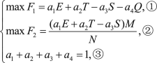  (15)

  where ① indicates the objective function 1 in a scenario with a strong communication anti-jamming capability; ${a_1}$, ${a_2}$, ${a_3}$ and${a_4}$ are the weighting coefficients, representing the effects of the jamming power suppression, system operational time, spatial aggregation penalty, and quantity penalty in the distributed communication jamming scheme, respectively, and they can be adjusted according to the specific needs of a jamming environment; ② stands for the objective function 2 in a scenario with a weak communication anti-jamming capability, which increases the penalty for a given number of jamming devices; namely, the penalty will decrease with the number of jamming devices, and the penalty will be enormous when the number of jamming devices is significantly smaller than the number of communication nodes; objective function 2 aims to improve the searching capability of the objective function for the optimal solution with a minimal number of jamming devices; ③ defines that the sum of the weights of the four evaluation indicators is one, which contributes to the intuitive presentation of the proportion of each weight.

MSPSGA algorithm model

Standard genetic algorithm

The standard genetic algorithm (SGA) denotes a stochastic optimization search method that mimics biological evolution in nature. The principle of the SGA is to search for good genes and guide the population evolution through encoding, selection, crossover, and mutation⁴⁷ to obtain an optimal solution. The SGA is simple and easy to implement and, thus, has been widely used in many fields, including combinatorial optimization, function optimization, and machine learning. However, it is time-consuming and performs poorly when scheduling the number of devices and power resources of a distributed communication interference system. In addition, its adaptability to different jamming scenarios is poor, and it has a high failure rate in scenarios with a small number of jamming devices.

MSPSGA

The MSPSGA divides the population into two populations, a master population and a slave population, and implements them in parallel according to different functions⁴⁸. The proposed MSPSGA, using a real number encoding, can directly process raw data and reduce the complexity of encoding and decoding⁴⁹. In addition, an individual in a population represents a candidate solution of the interference scheme, and it is initialized by roulette; the mutation mode denotes a local mutation, and the crossover mode is a one-way full replication. Each slave population operates independently, mutates, and evolves without cross-overing with other slave populations. The master population is generated by the crossover of historically optimal slave populations, which guides the power scheduling of slave populations. Also, the master population is updated and immediately adapted to all slave populations.

• (1) Power scheduling strategy. To address the problem that the SGA algorithm cannot efficiently schedule the interference power with constraints, this study proposes two strategies. In addition, to give the master population a guiding role over the slave population and to provide the slave population with a certain degree of flexibility, this study designs a master-slave power scheduling strategy. Based on the difference of the fitness of the objective function between the master population and each slave population, the probability of increasing or decreasing the power of any jamming device in the slave population was adjusted to realize the guided scheduling of interference power, where ${P_m}$ and ${P_s}$ denote the interference schemes of the master and slave populations, respectively;${P_{master}}$ and ${P_{slave}}$ represent the sums of the interference power within the master and slave populations, respectively; $ratio$ represents the middle value of the power scheduling; ${P_{ini}}$ and ${P_{ind}}$ are the probabilities of increasing and decreasing the power of a jamming device in the slave population by one level, respectively.

  The pseudo-code for the master-slave population-based power scheduling strategy is given in Algorithm 1.

  Algorithm 1: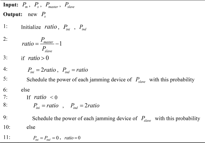

  

  Master-slave populated power scheduling strategy.

  After the jamming scheme has met the constraint of global jamming suppression, a fixed-position power scheduling strategy is used to reduce the redundant jamming power of individual jamming devices. The jamming scheme based on the master population fixed the deployment position, and iteratively compared the fitness of the objective function to reduce the maximum jamming power in the jamming equipment, so as to prolong the effective working time of the jamming system. In this strategy, ${f_{master}}$ represents the objective function fitness of the master population, and its pseudo-code is given in Algorithm 2.

  Algorithm 2: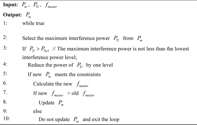

  

  Fixed-position power scheduling strategy.

• (2) Number scheduling strategy of jamming devices. A chromosome of the SGA algorithm represents a candidate solution, which can optimize only the jamming scheme of a fixed and known number of jamming devices. In order to effectively schedule a flexible number of jamming devices in the optimization of jamming resource scheduling, the number scheduling strategy of jamming devices is designed in this study. In the proposed strategy, ${N_i}$ represents the total number of iterations of the algorithm, $N{}_{c}$ is the scheduling index for the number of jamming devices, ${N_{slave}}$represents the number of jamming devices in the jamming scheme of the slave populations. If the master population fitness does not change in one iteration, $N{}_{c}$ is reduced by one, and the larger its value is, the more capable the algorithm is of jammers number searching. However, as the number of jamming devices increases, the number of poor solutions also increases. Therefore, generally, the number of jamming devices is selected as a quarter of the total number of iterations. The pseudo-code of the search number scheduling strategy is shown in Algorithm 3.

  Algorithm 3: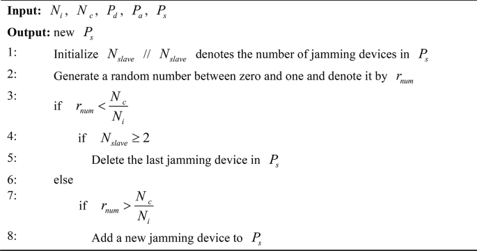

  

  Search number scheduling strategy.

  In Algorithm 3, ${p_d}$ represents the base probability of scheduling the number of jammers down, and ${p_a}$ is the base probability of scheduling the number of jammers up; therefore, the global number scheduling still works when the search number scheduling fails. The pseudo-code of the global number scheduling strategy is given in Algorithm 4.

  Algorithm 4: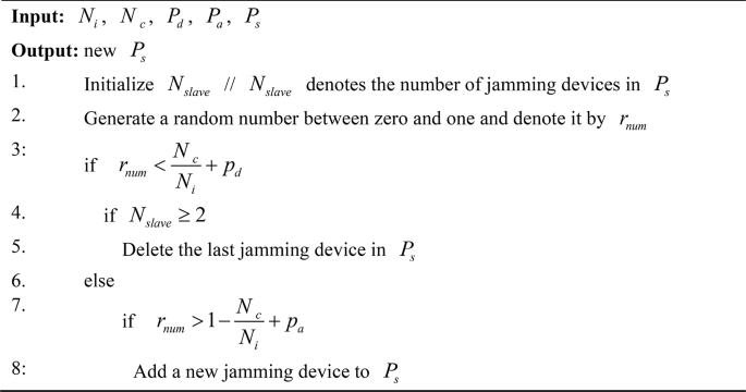

  

  Global number scheduling strategy.

• (3) Algorithm processing. Let ${N_{inow}}$ be the current iteration number of the MSPSGA and ${f_{slave}}$ be a slave population fitness. By integrating the advantages of the master-slave populated power scheduling strategy in enriching the diversity of sub-populations and frequently conducting guided power scheduling, as well as the advantage of the fixed-position power scheduling strategy in efficiently reducing redundant jamming power, and combining the advantage of the search number scheduling strategy with its significant effect in the early stage and the advantage of the global number scheduling strategy in adaptive and stable adjustment, the pseudo-code of the MSPSGA is shown in Algorithm 5.

  Algorithm 5: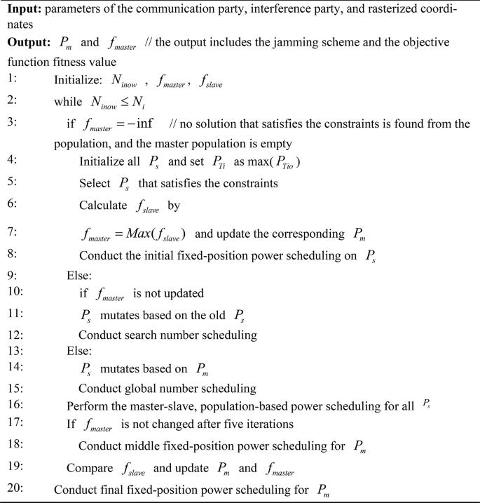

  

  Global number scheduling strategy.

  From the perspective of the whole function, the outer loop of MSPSGA is executed T times, and the inner loop within each outer loop is executed NP times. Therefore, the time complexity of MSPSGA is ${O_{({\text{T}} \times {\text{NP}})}}$. During the execution of the algorithm, the main parts occupying space are the data structures related to NP and the data that grows with the increase of T. Hence, the space complexity of MSPSGA is ${O_{({\text{T}}+{\text{NP}})}}$, where T represents the maximum number of iterations of the algorithm and NP represents the number of chromosome groups.

Results and discussion

Simulation parameter settings

In the experiment, an Intel(R) Core(TM) i5-8300 H CPU @ 2.30 GHz processor with 16.0 GB of RAM and an NVIDIA GTX1080Ti graphic card were used, and an environment of anaconda 23.7.4 was selected for verification.

In practical applications of communication clusters, all communication nodes are deployed around a certain area to achieve efficient inter-communication in a system. Based on this, a simulation area with a 26-km length and a 26-km width was defined and rasterized to form 1,300 × 1,300 intersections; the horizontal and vertical coordinates ranged from zero to 1299. The threat level of communication nodes, the forbidden radius of the jamming device deployment, and nodes’ coordinates were randomly generated. The maximum receiving power of a communication device was set to the maximum value of the receiving power between all the devices. The simulation parameters were set as follows: the antenna gain of jamming devices was 1.5 dB; the communication antenna’s gain was 4 dB; the height of jamming devices and communication antenna was fixed; the polarization loss of the jamming and communication signals was one; the filtering loss was 0.8; the threshold value of the jamming-to-signal ratio was set to three; the jamming devices’ battery capacity was 24 AH; the output voltage was 24 V; the full-time transmitting power of a non-jamming signal was 4 W. The effective operational threshold of the battery capacity was 0.95; the scaling factors were 1.0, 0.5, 3.0, and 12.0 in sequence. After setting the signal receiving power of a communication node, in a scenario with one jamming device and one communication node, the jamming signal transmitting power and the longest calculated statistical jamming distance were set, as shown in Table 1.

Table 1 Interference power and applicable distance settings.

Further, it was necessary to determine a feasible solution for the construction of a communication jamming environment in a short time to generate a distributed communication jamming scheme. Namely, a short convergence period and fast convergence speed were required, so the MSPSGA algorithm’s parameters were set accordingly, as presented in Table 2. In Table 2, T represents the maximum number of iterations, NP is the number of chromosome groups, M is the maximum number of available jamming devices, and N denotes the number of communication nodes.

Table 2 Parameter settings of the improved particle swarm algorithm.

Wireless communication nodes are often affiliated with multiple communicating parties. Multiple effective two-way communication links form a complex wireless communication network system. In this simulation experiment, 2 ultra-short wave communication nodes with a power of 50 watts and 10 ultra-short wave communication nodes with a power of 25 watts are designed for simulation. To serve and support communication users traveling along highways, communication nodes are often deployed along the surrounding areas of traffic roads, as shown in node deployments I (Fig. 2). To serve complex areas with large differences in the distribution density of communication users, the deployment of communication nodes often adopts a combination of overall concentration and scattered distribution at sporadic points, as shown in node deployments II (Fig. 3).

Fig. 2

Communication node deployment I.

Fig. 3

Communication node deployment II.

MSPSGA simulation verification and result analysis

The proposed MSPSGA was simulated and compared with the genetic particle swarm algorithm²³, the adaptive grid particle swarm algorithm⁵⁰, the genetic algorithm⁵¹, the simulated annealing algorithm⁵² and non-dominated sorting genetic algorithm III⁵³. The simulated annealing algorithm generated two new solutions after each iteration, and this algorithm was iterated 500 times. The settings of the other comparative algorithms were the same as that of the MSPSGA. The proposed algorithm is adaptable, and its algorithm steps, object function, and objective function’s weights can be adjusted to different operational modes. The objective function one performs a linear summation of the four weights. It gives equal emphasis to each item in model 1. For the high-speed countermeasure scenario with a fixed number of jamming devices, the fourth weight is removed. It can also be modified according to the characteristics of the application scenario. For example, removing weight three can achieve the spatial aggregation of low-power jamming devices. The objective function two reduces the usage of the number of jamming devices. Depending on the adjustment of the weight parameters, it can enhance the search ability of the jamming scheme with the minimum number of jamming devices. It can also focus more on the system operation duration or the jamming power suppression effect for the search. The objective function’s weights used in the experiments are shown in Table 3.

Table 3 Weights of the objective functions in different operational modes.

Minimum number of jamming devices search experiment

Experiment I with a fixed number of jamming devices was conducted to simulate and test the ability of the proposed algorithm to construct a communication jamming environment with a minimum number of jamming devices when jamming devices were scarce. Previous experiments have shown that when the number of jamming devices is three or four, there exist feasible solutions that meet the constraints for two communication node deployments. When the MSPSGA searched for interference solutions of the lowest number of jamming devices in Experiment 1, objective function 2 was used, and the number scheduling strategy and fixed-position power scheduling strategy of the master population at the initial and middle iterations were canceled to improve the algorithm’s search ability for feasible solutions and accelerate the iteration process. The experimental results are shown in Table 4; Fig. 4, where the statistical values of 30 independent runs of each algorithm are presented, (3) indicates that the MSPSGA algorithm has found a solution where the number of jamming devices is three.

Table 4 Scenario comparison results for the minimum number of jamming devices.

Fig. 4

Scenario comparison results for the minimum number of jamming devices.

The search ability of the comparison algorithms under the minimum number of jamming devices was significantly affected by the layout of the communication nodes to various degrees, and the increase in ability degree varied. The proposed MSPSGA had a high success rate in searching for the minimum number of jamming devices. In the scenario of communication node deployment II, where three jamming devices were used, the success rate of the proposed MSPSGA was 40% higher than that of the adaptive grid particle swarm algorithm. In addition, when the number of jamming devices increased from three to four, the success rate of the adaptive grid particle swarm algorithm increased from 30 to 86.6%, whereas the success rate of the proposed MSPSGA increased from 70 to 100%; also, MSPSGA was a 60% probability of obtaining a jamming solution with three jamming devices.

Maximum algorithm speed experiment

Experiment II was conducted in a high-speed countermeasure scenario. The large-scale construction of the communication jamming environment increased the demand for the number of jamming devices; the computational complexity significantly also increased, and the contribution rate of the system to the jamming effect required a high algorithmic speed. When there is no feasible solution, the running time of various algorithms is different from that of feasible solutions. In Experiment II, communication node deployment II was used to reduce the impact on statistics when there no feasible solution could be obtained. When the number of jamming devices for which the probability of having a solution was greater than 90%, each algorithm was run 15 times in turn, and the average solution data of the first 10 times was used for comparison. Since the number of jamming devices was fixed, the MSPSGA’s number scheduling strategy was canceled. The simulation comparison results of the algorithms are shown in Table 5; Figs. 5 and 6.

Table 5 Comparison results of the scenario with high-speed countermeasure.

Fig. 5

High-speed countermeasure I.

Fig. 6

High-speed countermeasure II.

The results indicated that the proposed algorithm had advances in the algorithm running time, average power of jamming devices, average maximum jamming power, and system operational time compared to the other algorithms. When the number of jamming devices was five, the running time of the proposed MSPSGA was 4% shorter than that of the simulated annealing algorithm; thus, the proposed algorithm was faster. When the number of jamming devices was nine, compared to the genetic particle swarm algorithm, the average power of the proposed MSPSGA was reduced by 73%, the maximum power was reduced by 85%, and the system’s operational time was extended by 309%; thus, the jamming system’s concealment, survivability, and operational time were improved.

Interference scheme generation experiment

Experiment III simulated an actual communication jamming scheme generation process. Since the existing algorithms cannot optimize the number of jamming devices, the method of manually traversing a certain number of interfering devices has been often used, and the interfering scheme with the highest fitness value has been typically selected for the number of jamming devices; however, this is not efficient. In contrast, the proposed algorithm innovatively employs a scheduling strategy for the number of jamming devices to enhance the algorithm’s search speed and reduce manual operation. To solve the problem of selecting the initial jammer, the simulation of experiment 3 is divided into two groups. The first group is the simulation experiment of traversing the initial jammer number, and the second group is the simulation experiment of randomly selecting the initial jammer number.

When communication node deployment I was used in Group 1, the five algorithms traversed the number of jamming devices from one to 12, the number of jamming devices corresponding to the algorithm with the highest fitness value was searched for three more times, and the interference scheme with the highest fitness value among the 15 interference schemes was selected as a final interference scheme. Moreover, three search modes for the objective function were tested: Mode 1 had balanced weights; Mode 2 focused on the operational time of a jamming system when the number of jamming devices was under control; Mode 3 focused on the jamming effect when the number of jamming devices was under control.

As displayed in Table 6, based on the experimental results of Group 1, in the case of a weak penalty for the number of jamming devices, the proposed algorithm operating in Mode 1 used a relatively large number of low-power jamming devices to form a distributed communication interference environment to improve the objective function’s fitness value, extend the system’s operational time, and improve the comprehensive effects of the interference scheme. In Mode 1, the MSPSGA used 140% redundancy of the number of jamming devices, improved the objective function fitness by 104%, decreased the total search time by 32%, reduced the average power by 71%, and extended the system’s operational time by 46% compared to the genetic algorithm.

Table 6 Comparison results of number scheduling scenario 1.

In Modes 2 and 3, the proposed algorithm optimized the number of jamming devices under the premise of controlling the number of jamming devices, focusing on the operational time and effectiveness of the jamming system, respectively. In Mode 2, compared to the adaptive grid particle swarm algorithm, the proposed MSPSGA improved the objective function’s fitness value by 1.9%, reduced the total algorithm running time by 54%, decreased the average power by 79%, and extended the system’s operational time by 200%. Thus, under the same number of jamming devices, all indicators were improved compared to the other algorithms. In Mode 3, compared to the genetic particle swarm algorithm, the MSPSGA reduced the number of jamming devices by 25%, increased the objective function’s fitness value by 26.7%, shortened the total running time of the algorithm by 54%, decreased the average power by 88%, and extended the system’s operational time by 300%, thus achieving the overall improvement of all indicators while preserving interfering resources. Compared with the simulated annealing algorithm, although the total time of the MSPSGA algorithm has been extended by 2.9%, it has obvious advantages in terms of the number of jamming devices, the fitness value of the objective function, the average power, and the system working time parameters. The proposed algorithm performed better in searching for an optimal interference scheme than the other algorithms using the search strategy of traversal and repetition.

In the experiments of Group 2, the proposed algorithm used the number scheduling strategy. When communication node deployment I was used, after setting the initial number of jamming devices, each algorithm was run 10 times in turn, and the average value was used for comparison. The comparison results are shown in Table 7. Compared to Mode 1, Modes 2 and 3 could effectively control the number of jamming devices. The ratio of the full range to the average value of the number of jamming devices deployed was 67% in Mode 1, 29% in Mode 2, and 19% in Mode 3. However, after applying the number scheduling strategy, the efficiency of the proposed algorithm in searching for the optimal interference scheme was higher than that of the search methods in Group 1 when only one iteration was performed; this proved the effectiveness of the number and power scheduling strategy. Further, the worst value of each indicator in the three operational modes of the proposed algorithm was compared with the best value of the comparing algorithms in Group 1 to verify the adaptability of the proposed algorithm to different initial numbers of jamming devices and operational modes. The results showed that the running time was reduced by 84%, the average power was reduced by 57%, and the system’s operational time was extended by 128%.

Table 7 Comparison results of number scheduling scenario 2.

Objective function comparison experiment

For distributed communication interference scenarios, there has been little research on the objective function that describes the distributed deployment of low-power communication jamming devices and the scheduling of interference resources. In this study, objective function 1 indicated the interference scenario with multiple jamming devices interfering with multiple communication nodes²². Similarly, objective function 2³³ referred to the interference scenario containing multiple jamming devices interfering with a radar network. Finally, objective function 3 corresponded to the scenario where an airborne interference node was interfering with the ground targets⁵⁴. The three functions are defined by Eqs. (16)–(18) based on the background and constraints used in this study.

$$\left\{ \begin{gathered} JS{R_j}={k_{yj}} \hfill \\ E=\sum\limits_{{j=1}}^{M} {{w_j}JS{R_j}} \hfill \\ \end{gathered} \right.$$

(16)

$$\left\{ \begin{gathered} JS{R_j}=\left\{ \begin{gathered} 1,{k_{yj}} \geqslant 6 \hfill \\ \frac{2}{3}(\frac{{{k_{yj}}}}{3} - 0.5){\log _3}{k_{yj}},6 \geqslant {k_{yj}}>3 \hfill \\ 0,{k_{yj}}<3 \hfill \\ \end{gathered} \right. \hfill \\ E=\sum\limits_{{j=1}}^{M} {{w_j}JS{R_j}} \hfill \\ \end{gathered} \right.$$

(17)

$$\left\{ \begin{gathered} JS{R_j}={k_{yj}} \hfill \\ E=\sum\limits_{{j=1}}^{M} {{w_j}} \hfill \\ \end{gathered} \right.$$

(18)

For communication node deployment I with a fixed initial number of jamming devices was used in the analysis. The proposed MSPSGA operating in Mode 1 with objective function 1 and Mode 3 with objective function 2 was compared with the above three objective functions. The five objective functions were run independently 10 times, and their average values are shown in Table 8; Figs. 7, 8 and 9.

Table 8 Objective function comparison results.

Fig. 7

Optimal number.

Fig. 8

Average power.

Fig. 9

Operational time.

The results in Table 8 show that the searching ability of the number of jamming devices and the system’s operational time of the ob31.66jective functions in the interference scenario showed a clear downward trend with the number of jamming devices; namely, the scheduling ability of the number and power of jamming devices was poor. Objective function 2 had a 93% decrease in the full range of Optimal number compared to the first objective function for comparison; the full range of system operational time showed a 79% decrease compared to the third objective function for comparison. The average power did not differ significantly for different objective functions when the number of jamming devices barely met the jamming requirement. However, when the number of jamming devices had a certain redundancy, the power scheduling capability of the compared objective functions decreased significantly. For objective function 2, when the number of jamming devices was eight, the average power was 52% lower than that of the second objective function for comparison, but when the number of jamming devices was 12, it was 69% lower than that of the first objective function for comparison. In summary, under the condition of controlling the interference power, objective function 1 used a relatively large number of jamming devices to construct a complex interference environment with an acceptable cost. In addition, objective function 2 was less affected by the initial setting of the number of jamming devices, and its ability to use the minimum number of jamming devices, a low interference power, and a long system operational time to construct a communication interference environment was stable and convergent.

Conclusion and future scope

In this paper, two multi-objective optimization models of the number and operational time of distributed communication jamming are developed to optimize the four jamming effects using three optimization variables. The constraints on the deployment of jamming devices, suppression of communication nodes, and continuous operation of jamming devices are defined, and a logarithmic stepped signal-to-noise ratio suitable for distributed communication jamming is determined. Finally, the improved MSPSGA with four strategies is proposed.

The results of the simulation experiments show that compared to the adaptive grid particle swarm algorithm, genetic particle swarm algorithm, genetic algorithm, and simulated annealing algorithm, the proposed algorithm performs well in finding the minimum number of jamming devices and is stable and reliable in the scenario with high-speed countermeasures. Using the optimal interference scheme, the optimal jamming solution can be rapidly obtained without relying on the initial setting of the number of jamming devices. The two proposed scheduling strategies, for the number and power, are in line with the requirements for flexible number and power of distributed communication jamming. Compared to the objective functions of multiple jamming devices targeting a networked radar, jamming devices targeting ground nodes, and multiple jamming devices targeting multiple communication nodes, the objective functions used in this study can save interference power. Objective function 1 focuses on the deployment of a large number of low-power jamming devices, whereas objective function 2 focuses on stable deployment with minimum interference resources.

In future research, the game confrontation of communication jamming and anti-jamming could be studied, and communication nodes with anti-jamming measures, such as frequency hopping, maneuvering, and concealment, could be explored. In addition, distributed interference equipment that can achieve scheduling under interference scenarios with highly dispersed spatial distribution, complex terrain, and air-ground coordination could be considered. The algorithms for such equipment could be integrated and developed using multi-agent and deep learning technologies to handle complex multi-variable large-scale interference resource joint scheduling.

References

Yuan, H. et al. Time-frequency analysis and type identification of high-density communication countermeasure electronic signals. Trait Signal. 39, 723–729 (2022).
Zheng, S., Zhang, C., Hu, J. & Xu, S. Radar-jamming decision-making based on improved Q-learning and FPGA hardware implementation. Remote Sens. 16, 1190 (2024).
Lei, T., Qilun, Z., Dongxi, W., Dong, Q. & Jinlu, H. & Ren, Z. Escort strategy based on loyal wingman in denial environment. J. Beijing Univ. Aeronaut. Astronaut. 47, 1058–1067 (2021).
Russell, S. AI weapons: Russia’s war in Ukraine shows why the world must enact a ban. Nature 614, 620–623 (2023).
Russell, S., Hauert, S., Altman, R. & Veloso, M. Ethics of artificial intelligence. Nature 521, 415–416 (2015).
Adam, D. Lethal AI weapons are here: How can we control them? Nature 8012, 521–523 (2024).
Li, Y. & Liang, S. Research on modulation recognition of underwater acoustic communication signal based on deep learning. J. Phys. Conf. Ser. 2435, 012007 (2023).
He, G. et al. Design and verification of assessment tool of shortwave communication interference impact area. Atmosphere 14, 1728 (2023).
Ravindran, M. A. et al. A novel technological review on fast charging infrastructure for electrical vehicles: Challenges, solutions, and future research directions. Alexand. Eng. J. 82, 260–290 (2023).
Wang, X., Huang, T. & Liu, Y. Resource allocation for random selection of distributed jammer towards multistatic radar system. IEEE Access. 9, 29048–29055 (2021).
Li, S., Liu, G., Zhang, K., Qian, Z. & Ding, S. DRL-based joint path planning and jamming power allocation optimization for suppressing netted radar system. IEEE Signal. Proc. Lett. 30, 548–552 (2023).
Zhang, D., Sun, J., Yi, W., Yang, C. & Wei, Y. Joint jamming beam and power scheduling for suppressing netted radar system. In 2021 IEEE Radar Conference, 1–6 (2021).
Lu, D. J., Wang, X., Wu, X. T. & Chen, Y. Adaptive allocation strategy for cooperatively jamming netted radar system based on improved cuckoo search algorithm. Def. Technol. 24, 285–297 (2023).
Xin, Q., Xin, Z. & Chen, T. Cooperative jamming resource allocation with joint multi-domain information using evolutionary reinforcement learning. Remote Sens. 16, 1955 (2024).
Yao, Z., Tang, C., Wang, C., Shi, Q. & Yuan, N. Cooperative jamming resource allocation model and algorithm for netted radar. Electron. Lett. 58, 834–836 (2022).
Jin, W. C., Kim, K. & Choi, J. W. Adaptive jamming considering location information inaccuracy for anti-UAV system. In 2021 International Conference on Information Networking, 480–482 (2021).
Xiong, M., Zhuo, J., ,Dong, Y. & Jing, X. A layout strategy for distributed barrage jamming against underwater acoustic sensor networks. J. Mar. Sci. Eng. 8, 252 (2020).
Wu, Z., Luo, Y. & Hu, S. Optimization of jamming formation of USV offboard active decoy clusters based on an improved PSO algorithm. Def. Technol. 32, 529–540 (2024).
Rao, N. et al. Joint optimization of jamming link and power control in communication countermeasures: A multiagent deep reinforcement learning approach. Wirel. Commun. Mob. Com. 1, 7962686 (2022).
Wu, L. et al. A. UAV-assisted maritime legitimate surveillance: Joint trajectory design and power allocation. IEEE Trans. Veh. Technol. 72, 13701–13705 (2023).
Tang, C., Ding, J. & Zhang, L. LEO satellite downlink distributed jamming optimization method using a non-dominated sorting genetic algorithm. RemoteSens 16, 1006 (2024).
DeJiang, L., Wang, W., You, C. & Xing, H. Adaptive scheduling method of joint multi-resource for cooperativeinterference of networked radar system. Syst. Eng. Electron. 45, 2744–2754 (2023).
Zekun, Y., Chao, W., Qingzhan, S., Shaoqing, Z. & Naichang, Y. Cooperative jamming resource allocation model for radar network based on improved discrete simulated annealing genetic algorithm. Syst. Eng. Electron. 46, 1–8 (2024).
Jiechen, X. Research on decision algorithm for cooperative interference against radar net. Master’s thesis, Harbin Engineering University (2022).
Xin, X., Gaogao, L., Qiang, L. & Dongjie, H. Distributed interference optimal array method for sidelobe cancellation. Syst. Eng. Electron., 1–8 (2024).
Xing, H. X., Wu, H., Chen, Y. & Wang, K. A cooperative interference resource allocation method based on improved firefly algorithm. Def. Technol. 17, 1352–1360 (2021).
Xixing, H., Huaxingng, Q. & Wang, K. A joint allocation method of multi-jammer cooperative jamming resources based on suppression effectiveness. Mathematics 11, 826 (2023).
Chen, P., Li, H. & Ma, L. Distributed massive UAV jamming optimization algorithm with artificial bee colony. IET Commun. 17, 197–206 (2023).
Wu, Z., Hu, S., Luo, Y. & Li, X. Optimal distributed cooperative jamming resource allocation for multi-missile threat scenario. IET Radar Sonar Navig. 16, 113–128 (2022).
Zhang, P., Huang, Y. & Hejin, Z. An electronic jamming method based on a distributed information sharing mechanism. Electronics 12, 2130 (2023).
Ye, F., Li, X., Jiang, T., Li, Y. & Li, Y. Research on jamming decision making based on feedback iterative-brown algorithm. In 2020 IEEE USNC-CNC-URSI North American Radio Science Meeting, 3–4 (2020).
He, B. & Su, H. Game theoretic countermeasure analysis for multistatic radars and multiple jammers. Radio Sci. 56, 1–14 (2021).
Zhang, Y. et al. Jamming policy generation via heuristic programming reinforcement learning. IEEE Trans. Aerosp. Electron. Syst. 59, 8782–8799 (2023).
Zhang, W., Ma, D., Zhao, Z. & Liu, F. Design of cognitive jamming decision-making system against MFR based on reinforcement learning. IEEE Trans. Veh. Technol. 72, 10048–10062 (2023).
Rao, N., Xu, H., Jiang, L., Song, B. & Shi, Y. Allocation algorithm of distributed cooperative jamming power basedon multi-agent deep reinforcement learning. Acta Electron. Sin. 06, 1319–1330 (2022).
Li, X. et al. Distributed multi-agent interference coordination in native AI enabled multi-cell networks for 6G. In 2023 26th International Symposium on Wireless Personal Multimedia Communications,8–13 (2023).
Ning, R., Hux, X. & Jialin, S. Q-learning intelligent jamming decision algorithm based on efficient upper confidence bound variance. J. Harbin Inst. Technol. Engl. Ed. 54, 162–170 (2022).
ZhuanSun, S., Yang, J. A. & Liu, H. An algorithm for jamming strategy using OMP and MAB. Eurasip J. Wirel. Comm. 85, 1 (2019).
Hua, X., Bailin, S., Lei, J., Ning, R. & Yunhao, S. An intelligent decision-making algorithm for communicationcountermeasure jamming resource allocation. J. Electron. Inf. Techn Sin. 11, 3086–3095 (2021).
Bailin, S., Hux, X., Zisen, Q., Ning, R. & Peng, P. A collaborative communication Jamming decision algorithm based on deep reinforcement learning. Acta Electron. Sin. 06, 1301–1309 (2022).
Liu, Z., Wang, X., Kang, W. & Chen, Y. Research on multi-UAV collaborative electronic countermeasures effectiveness method based on CRITIC weighting and improved gray correlation analysis. AIP Adv., 14 (2024).
Zhang, S. et al. Design and implementation of reinforcement learning-based intelligent jamming system. IET Commun. 14, 3231–3238 (2020).
Xiang, P., Hua, X., Lei, J., Yue, Z. & Ning, R. A. Dynamic adaptive jamming power allocation method based on deep reinforcement learning. Acta Electron. Sin. 05, 1223–1234 (2023).
Liu, L. et al. GIS and cellular automata based slope rainwater movement process model and its application. Sci. Rep. 14, 9750 (2024).
Maimistov, A. I. Propagation of electromagnetic waves in a nonlinear hyperbolic medium. Bull. Ledev Phys. Inst. 50, S1066–S1074 (2023).
Kuang, Z., Pan, Y., Yang, F. & Zhang, Y. Joint task offloading scheduling and resource allocation in air-ground cooperation UAV-enabled mobile edge computing. IEEE Trans. Veh. Technol. 73, 5796–5807 (2023).
Kumar, B. A. et al. Hybrid genetic algorithm-simulated annealing based electric vehicle charging station placement for optimizing distribution network resilience. Sci. Rep. 14, 7637 (2024).
Skorpil, V. & Oujezsky, V. Parallel genetic algorithms’ implementation using a scalable concurrent operation in python. Sensors 22, 2389 (2022).
Salih, K. M. & Shakir, M. A. Optimization algorithms used in cognitive radio networks: An overview. In 2022 International Conference on Computer Science and Software Engineering, 201–206 (2022).
Han, Y. et al. Design and application of vague set theory and adaptive grid particle swarm optimization algorithm in resource scheduling optimization. J. Grid Comput. 21, 24 (2023).
Tossa, F., Abdou, W., Ansari, K., Ezin, E. C. & Gouton, P. Area coverage maximization under connectivity constraint in wireless sensor networks. Sensors 22, 1712–1712 (2022).
Yang, L. S., Wen, B. & Yan, J. J. Network site optimization and clustering study based on simulated annealing algorithm. IEEE Access. 11, 108167–108177 (2023).
Agnihotri, S. & Dhodiya, J. M. Non-dominated sorting genetic algorithm III with stochastic matrix-based population to solve multi-objective solid transportation problem. Soft Comput. 27, 5641–5662 (2022).
Xicheng, D. Research on electromagnetic signal situational awareness blind area air-land coordination coverage algorithm. Master’s thesis, Graduate School of National University of Defense Technology (2022).
Author information
Authors and Affiliations
Contributions
Z.W. proposed a design plan; W.W. and Z.Z. conducted experimental simulations; Z.W. and W.W. wrote the manuscript; J.Z. provided guidance on the experiments and did the final revi-sion of the manuscript completed by Z.W. and W.W.; J.Z. provided guidance on the experi-ments and did the final revision of the manuscript.
Corresponding author
Ethics declarations
Competing interests
The authors declare no competing interests.
Additional information
Publisher’s note
Springer Nature remains neutral with regard to jurisdictional claims in published maps and institutional affiliations.
Rights and permissions
Open Access This article is licensed under a Creative Commons Attribution-NonCommercial-NoDerivatives 4.0 International License, which permits any non-commercial use, sharing, distribution and reproduction in any medium or format, as long as you give appropriate credit to the original author(s) and the source, provide a link to the Creative Commons licence, and indicate if you modified the licensed material. You do not have permission under this licence to share adapted material derived from this article or parts of it. The images or other third party material in this article are included in the article’s Creative Commons licence, unless indicated otherwise in a credit line to the material. If material is not included in the article’s Creative Commons licence and your intended use is not permitted by statutory regulation or exceeds the permitted use, you will need to obtain permission directly from the copyright holder. To view a copy of this licence, visit http://creativecommons.org/licenses/by-nc-nd/4.0/.
About this article
Cite this article
Wei, Z., Wu, W., Zhan, J. et al. Distributed communication interference resource scheduling using the master-slave parallel scheduling genetic algorithm. Sci Rep 15, 3431 (2025). https://doi.org/10.1038/s41598-025-86478-x
Received:
Accepted:
Published:
DOI: https://doi.org/10.1038/s41598-025-86478-x