
Abstract
We introduce an operational definition of the Berry Phase Rectification Tensor as the second order change of polarization of a material in response to an ideal short pulse of electric field. Under time reversal symmetry this tensor depends exclusively on the Berry phases of the Bloch bands and not on their energy dispersions, making it an intrinsic property to each material which contains contributions from both the inter-band shift currents and the intra-band Berry Curvature Dipole. We also introduce the Solar Rectification Vector as a technologically relevant figure of merit for bulk photo-current generation which counts the number of electrons contributing to the rectified current per incoming photon under ideal black-body radiation in analogy with the classic solar cell model of Shockley and Queisser. We perform first principle calculations of the Berry Phase Rectification Tensor and the Solar Rectification Vector for the Weyl semi-metal TaAs and the insulator LiAsSe2 which features large shift currents close to the peak of solar radiation intensity. We also generalize the formula for the Glass coefficient to include the spectral distribution of the incoming radiation, the directionality dependence of the conductivity of the material and the reflectivity at its surface.

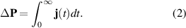
Original content from this work may be used under the terms of the Creative Commons Attribution 4.0 license. Any further distribution of this work must maintain attribution to the author(s) and the title of the work, journal citation and DOI.
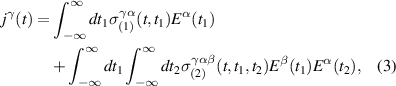
1. Introduction
Several remarkable relations between the quantum geometry and topology of electronic states in crystalline solids and their non-linear optical and transport properties have been unraveled over the last few decades. One of the second order effects intimately intertwined with the geometry of electronic wave-functions is the shift current [1–10], which is a rectified current arising in response to AC electric fields that drive optical transitions in crystals without inversion symmetry. The shift current arises from band-off-diagonal components of the velocity operator, in contrast to the injection current, which arises from the band-diagonal difference of group velocities between empty and occupied states [2, 3, 5–10]. In materials with time reversal symmetry (TRS), the shift current differs from the injection current in that only the shift current can lead to rectified currents in response to linearly polarized electric fields, making it attractive for photovoltaic applications [6, 11–14] since it can lead to a DC current for electric fields with no net degree of circular polarization such as those arriving from the Sun.
Another second order effect with an intimate connection to the geometry of electronic wave functions is the non-linear Hall effect driven by the Berry curvature dipole (BCD) [10, 15–17], that has been recently observed experimentally [18–23]. Like the shift current, the BCD non-linear Hall effect can also give rise to a rectified current in response to a linearly polarized electric field, but with the crucial difference that this effect occurs only in metals at low frequencies in a Drude-like fashion [10]. These two distinct effects, however, appear to have a connection, as suggested by the quantum-rectification sum rule (QRSR) derived in [10]. The QRSR states that the frequency integral of the total rectification conductivity for any time-reversal-invariant material is completely independent of energy dispersions and entirely controlled by the quantum geometric Berry connections of the bands. The contributions to the QRSR arise from the BCD effect, which accounts for all the intra-band weight in a Drude-like peak, and the shift current, which accounts for all the inter-band contributions. In contrast, injection currents do not contribute to the QRSR under time reversal invariant conditions.
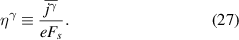
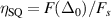
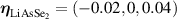
In this work, we will show that the QRSR defines a three-index Berry phase rectification tensor (BPRT), which depends only on the Berry phase geometry of a time-reversal-invariant material. In d-dimensions the BPRT has units of , and therefore, it is dimensionless for 3D materials. We will introduce an operational definition of the BPRT by considering the change of polarization in response to ideal short pulses of electric fields (see figure 1) and compute it from first principle calculations for the Weyl semi-metal TaAs [24–27] and demonstrate that, remarkably, the net contribution from the BCD [28] is comparable to the inter-band contribution from shift currents. We will also compute the BPRT for the insulator LiAsSe2, which is a promising photo-voltaic material [6]. Additionally we will introduce the notion of the solar rectification vector (SRV), whose magnitude serves as a technologically useful figure of merit for bulk photo-current generation, and is defined from the average DC current produced under ideal black-body solar radiation, analogous to the model employed by Shockley and Quessier (SQ) in their seminal study of p-n junction solar cells [29]. We will demonstrate that LiAsSe2 could generate photo-currents as large as 5 mA cm−2, which is about 5% of the ideal maximum from the SQ model [29]. The direction of the SRV for these materials is shown as a yellow vector in figure 2.


Figure 1. The Berry phase rectification tensor measures the second order change of polarization (which equals the area in the right panel) in response to delta function pulse of electric field (left panel).
Download figure:
Standard image High-resolution image
Figure 2. Crystal structures and solar rectification vectors (SRV) for (a) LiAsSe2 and (b) TaAs.
Download figure:
Standard image High-resolution imageAs we will illustrate, one of the appealing features of our formulas for computing the BPRT and the SRV, is that they can be readily combined with realistic first principle calculations of material band structures. Therefore, these formulas have the potential to be used to implement a more comprehensive and systematic search of materials with technologically desirable bulk photovoltaic properties.
2. The Berry phase rectification tensor
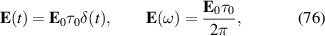
Consider an electronic system which is in equilibrium for , and at t = 0 is subjected to a quench of the vector potential, leading to a delta-function pulse in the electric field of the form:


where Θ(t) is the heavy-side function. After the pulse, the net change of electric polarization can be obtained from:
This protocol is illustrated in figure 1. To second order in electric fields the current is related to the linear and second order conductivity as:
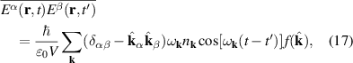
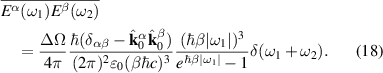
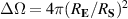
where Greek letters denote space indices and here and throughout the paper sum over repeated indices is understood unless otherwise stated. Therefore, the expansion of the polarization in powers of A0 is:
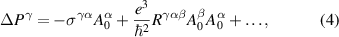
where is the zero frequency linear conductivity, and defines the BPRT of the system, which is given by (see appendix


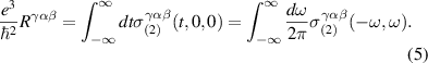
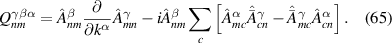
Equation (4) expresses the notion that the BRPT measures the net displacement of the average position of an electronic system to second order in the strength of delta function pulse in electric field. As demonstrated in [10] for the ground state of any non-interacting system with a time-reversal-invariant band structure, only contains information about the Berry connections of the bands. Specifically, in the clean limit of a time reversal invariant band structure, it is given by:


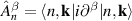
where , is the abelian Berry curvature of the nth band, and is the off-diagonal non-Abelian Berry connection and average is defined as:

where fn is the Fermi–Dirac occupation function of the nth Bloch band. The first term in equation (6) arises from the intra-band BCD while the two other terms arise from the inter-band shift current. Therefore the BPRT connects these two effects and allows for a concrete measure of the shift current effect, as a collective displacement of average position of the electron system in response to an electric field pulse. Such an interpretation of the BPRT suggests that time domain spectroscopic techniques [30, 31] are promising tools to measure the BPRT in materials. By construction the BPRT is symmetric in its last two indices, and the BCD does not contribute to fully diagonal components of the form . For a related, but more restricted, sum rule see [32].

Notice that the intra-band contribution to the BPRT, namely the Berry dipole contribution proportional to in equation (6), is gauge invariant as it only depends on the gauge invariant Berry curvature. Since the full BPRT tensor is also gauge invariant [10], it follows that the remainder of the tensor is separately gauge invariant. This remainder contains the contributions of inter-band transitions arising from shift-current effects [10]. Therefore, there is no gauge ambiguity in separating the intra- and inter-band contributions to the BPRT, and we will compute them separately for the semimetal TaAs in section 5.

3. The solar rectification vector
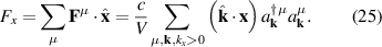
In this section we introduce a figure of merit for bulk photovoltaic materials that captures their amount of DC current generated from Sun-light under ideal conditions, and therefore it is a more relevant quantity for technological applications. Consider an statistical ensemble electric fields that is time-translationally invariant, whose average and two-time autocorrelation functions are given by:

Now, from equation (3), it follows that the ensemble averaged current is given by:

Then the average current will be time independent and given by:
Where is the Fourier transform of the electric field auto-correlation function. In the next subsection, we will compute such electric field auto-correlation function for the ensemble of solar black-body radiation.

3.1. Autocorrelations for black-body radiation
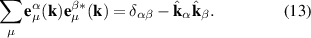
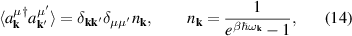
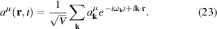
The photon eigenmode representation of the electric field operator in Heisenberg representation and residing in a periodic box of volume V is:
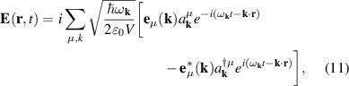
where , , are photon destruction and creation operators satisfying standard commutation relations, µ = x, y labels the directions of light polarization and the unit vectors satisfy:


The quantum ensemble average of the photon number is given the by the Planck distribution:
where β = 1/kB T is the inverse temperature of the black body. To compute the auto-correlation function of the electric field we use the following prescription for quantum-to-classical conversion of the averages:

Where in the left-hand side we have the correlations denoted by an over-bar, in which the electric field is viewed as a classical field, and in the right-hand side we have quantum mechanical averages in which the electric field is viewed as the operator appearing in equation (11). We have added a normal ordering of the quantum electric fields which removes the vacuum Casimir-type fluctuations which should be negligible in the thermodynamic limit . With this we obtain:

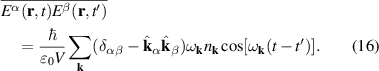
In the above formula all modes of light contribute to produce a fully isotropic correlator of electric fields at a given point r. This would be the situation if the point of interest was fully immersed inside the isotropic black-body radiation ensemble. However, when the radiation that arrives at r is highly directional we can modify the formula above by a one with an extra weighing function inside the momentum integral :

which phenomenologically takes into account the preferred directionality of the incoming light at a given point r. In the special case in which the function only for a very small region of solid angles, ΔΩ, around a specific direction , we have that:


For the light emitted from the Sun and arriving on earth, and would correspond to the unit vector defining the direction from Sun to earth, is the radius of the Sun, and is the distance of the Sun to the earth.


The formula above is expected to describe the ideal solar radiation before entering the earth atmosphere, but the solar irradiance spectrum on the surface of earth can still be reasonably well approximated by it (see e.g. [33]). Upon entering the atmosphere the spectral intensity gets reduced at specific frequencies corresponding to absorption of molecules in the atmosphere. There will also be a randomization of the transversality of the electric field due to elastic scattering. This could be accounted for by averaging the projector over some distribution of , but for simplicity we will simply replace the transverse projector in equation (18) by a delta function with all components of the electric field, namely we take the electric field correlator to be:

As we will see in the section 3.2, as along as the material is oriented so that its 'solar rectification vector' (to be defined in next subsection) is orthogonal to , one obtains the same current from the equation (19) as the one one would obtain from the equation (18) that takes into account the transverse nature of incident light.

Therefore, in conclusion, the electric field auto-correlation function associated with solar radiation, and which is needed in order to compute the average DC current in equation (10), can be written as:
where is the dimensionless Planck spectral distribution function, is the inverse temperature of the Sun TS ≈ 5778K, is the radius of the Sun, and is the Sun-earth distance. As we will see in the next subsection, the geometric factor will disappear from the normalized figure of merit that measures the electric current normalized to the incoming photon flux. They are needed however if one would like to compute the actual magnitude of the induced photo-current.


3.2. Definition of solar rectification vector
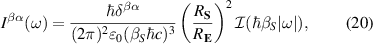
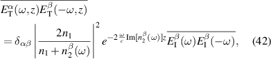
Equations (10) and (20) provide the total current density induced by exposing a material to solar radiation. To define a figure of merit for current generation, it is convenient to normalize such total current density (number of electrons per unit area per unit time) by the photon flux Fs (number of photons per unit area per unit time ), so as to count how many current-carrying electrons are induced per incoming photon. Let us therefore also compute the photon flux on earth. The photon density, n is given by:
![$[F_s] = m^{-2} s^{-1}$](https://content.cld.iop.org/journals/0022-3727/54/40/404001/revision3/dac118fieqn31.gif)

The photon current can be obtained from the continuity equation for photon density:

Which leads to the following expression for the photon current per unit of area per unit time:
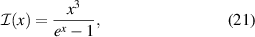
The expression above would give us the number of photons moving on a single direction (e.g. toward the right) on a given surface of a black-body, which can be pictured to be the surface of the Sun. On the surface of the Earth the photon flux is given by:

here ζ is the Riemann zeta-function.
Therefore, we define a three-component vectorial figure of merit called the SRV, and denoted by (γ = x, y, z), as the ratio of the electric current density and the photon flux, given by:

Notice that the SRV defined above depends only on the temperature of the Sun and the intrinsic rectification properties of the material. By combining equations (18) and (26) with the definition from equation (27), one arrives at the following explicit form of the SRV:

Where is defined in equation (21). We see that is a dimensionless vector for 3D materials and its magnitude, , counts the number of electrons contributing to the rectified current per incoming photon, therefore serving as a dimensionless figure of merit for the ideal bulk photo-current generated by a material under short-circuit configurations. Because the Planck distribution has vanishing intensity at small frequency, in the clean limit, the BCD Drude-like peak does not contribute to the rectified current and all the contributions arise from shift currents in time-reversal invariant materials, while injection current contributions vanish (see appendix


It is instructive to contrast this figure of merit with a comparable figure of merit for current generation for the ideal model of a p-n junction solar-cell proposed by SQ [29]. In the most ideal version of the SQ model one assumes that every photon with energy above the band-gap is absorbed and generates an electron and a hole that are successfully collected at opposite electrodes contributing to the current generation of the material. Therefore in the SQ model the total current density is:

Here is the analogue of the magnitude of the SRV, but defined for a conventional solar cell within the SQ model, and simply measures fraction of incident photons that have energy above the band-gap and thus can be absorbed by the material. The flux of such photons with energies above the band-gap, Δ0, can be computed in an analogous fashion to the total photon flux but inserting an extra factor to enforce that their energy is larger than Δ0, as follows:

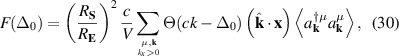
where Θ is the Heaviside function. The ratio of absorbed photons, , in equation (29), can thus be obtained as . SQ were primarily interested in optimizing the total power delivered by the solar cell and not the total current. It is however clear that the maximum current density is attained for which is achieved in the limit of vanishing gap. As we will see LiAsSe2 has a value of η = 0.05, and thus can produce a photocurrent that is 5% of the ideal SQ limit, in which every incoming photon produces an electron and a hole that do not recombine and are successfully captured at opposite electrodes contributing to the net current.


4. Material penetration
Our discussion of photo-current generation so far has assumed that light propagates inside the material as it would do in vacuum. This is a reasonable approximation only if the incoming radiation is not substantially modified inside the material. This can be justified for example if the material is much thinner than the decay length for light absorbtion in the material, , where λin is the typical wavelength of the incoming radiation and n is the complex index of refraction of the material. However, a more realistic calculation of the photo-current would include the frequency dependence of light absorbtion and propagation in the material, which is often accounted for by the Glass coefficient [11, 34].
![$L \sim \lambda_{in}/\mathrm{Im}[n]$](https://content.cld.iop.org/journals/0022-3727/54/40/404001/revision3/dac118fieqn40.gif)
In this section we take into account that the intensity of electric field decays inside the material, and derive the expression for the total current. For simplicity, we assume that incident radiation is normal to the solar cell surface so that that the electric field is parallel to the surface, namely along the XY plane in figure 4, and that the induced photo-current also flows along this XY plane. To estimate the electric field penetration, we use linear response theory. The geometry of the problem is shown in figure 4, and by the standard procedure of boundary condition matching from Maxwell equations (see e.g. [35]) leads to the following equations:


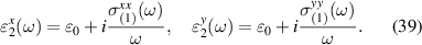
For simplicity we assume the magnetic permitivities of the vacuum and the bulk photovoltaic material to be frequency independent constants. We also assume that the material has a point group so that its linear conductivity is diagonal in its set of principal axes, and we take one these axes to be the z-axis that coincides with the direction of incoming light. The frequency dependence of these diagonal components of the linear conductivity of the material can be obtained from standard linear response theory [10, 32] and are given by:

where Γ is relaxation rate and  n
is the nth Bloch band energy dispersion. In the expression above β index is not summed over. From the above one can obtain the dispersion relations of light outside and inside the material to be:
n
is the nth Bloch band energy dispersion. In the expression above β index is not summed over. From the above one can obtain the dispersion relations of light outside and inside the material to be:

By taking into account standard electromagnetic boundary conditions [35], we can obtain the following relation describing the transmitted, , component of the electric field inside the material for a given incident component, :


Since the above relation between transmitted and incoming light is linear, we can compute ensemble averages of the transmitted electric field from the known ensemble averages of the incoming electric field. We take the ensemble average of the incoming electric field to be that of the ideal black-body radiation from equation (18), where we keep track explicitly of the transverse character of incoming light. From this it follows that the electric field auto-correlation function inside the bulk of the solar cell is:
where in the above expression the repeated indices are not being summed over and indices are understood to take only (x, y) components. Thus the total current is:

where W is the width of the sample, is the complex index of refraction from equation (41), and is given in equation (20). The formula above generalizes that from [11, 34] by adding the frequency dependence of the reflection coefficient at the material surface, the spectral distribution of incident light as well as the directional dependence of the conductivity of the material. We expect it to provide accurate estimates for realistic bulk-photovoltaic solar cell devices.


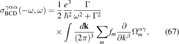
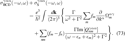
5. Bulk rectification of TaAs and LiAsSe2
In this section we combine our general considerations with first principle calculations of the non-linear opto-electronic properties of the 3D Weyl semi-metal TaAs and the insulator LiAsSe2. Because it is semi-metallic, TaAs has BCD and shift current contributions whereas LiAsSe2 only has shift current contributions. Our primary interest in TaAs is to investigate the interplay between the intraband BCD and interband shift-currents to its BPRT, although we also compute its SRV, while in the case of LiAsSe2 our primary interest is the estimation of its SRV due to its promise as a photovoltaic material, but we also compute its BPRT. Throughout this section we will be using the ideal formalism that neglects the modification of the incoming radiation inside the material, namely we will compute the BPRT and SRV from equations (6) and (27), respectively.
The band structures of LiAsSe2 and TaAs were calculated by the full-potential local-orbital [36, 37] minimum-basis code with the experimental crystal structure. Details of the calculations of band structure, Berry phases and non-linear rectification conductivity in the clean limit are presented in appendix
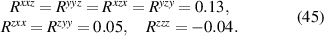
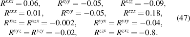
The values above contain the contribution from BCD and shift currents. The BCD part of the contribution to BPRT is:
Therefore, remarkably, we see that in spite of having all its spectral weight localized in a delta function Drude-like peak, in TaAs the BCD contributes to the net rectification tensor with a magnitude that is comparable with the net contribution from shift currents, and sometimes they have opposite signs as it is the case for the . The SRV for TaAs has a single non-trivial component , which is oriented along its polar axes as depicted in figure 2(a).

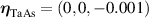

Figure 3. The non-zero conductivity components for LiAsSe2 as a function of frequency in the clean limit (Γ = 0). The dashed line is the solar Planck intensity distribution (in arbitrary units) showing its good overlap with the rectification conductivity of LiAsSe2.

Download figure:
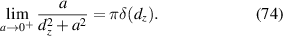
Standard image High-resolution image
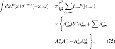
Figure 4. Illustration of the geometry for incident (I), transmitted (T) and reflected (R) light at the solar cell. For simplicity, we considered the light to be perpendicular to the surface. At the interface (solid black line) between vacuum (region 1) and the bulk photovoltaic material that makes the solar cell (region 2) the incoming light (I) splits onto reflected (R) and transmitted (T). The transmitted component generates the current J. µ0 is magnetic permitivity and 1, are permittivities of vacuum and the bulk photo-voltaic material respectively.

Download figure:
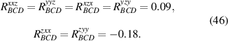
Standard image High-resolution imageOn the other hand, the lower Cc space group symmetry of LiAsSe2 allows for a larger set of independent components:
The SRV has two components , with the higher SRV magnitude η = 0.05, or in other words, it produces a photocurrent that is is 5% of the ideal limit for p-n junction solar cells.
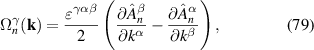
6. Discussion
We have introduced an operational definition of the BPRT as the second order polarization response of a material to an ideal delta function pulse of applied electric field. In the case of a time reversal invariant band structure this tensor is an intrinsic property of the material which only depends on the Berry connections of the Bloch bands and not on their energies. This tensor contains intra-band contributions which arise from the BCD and inter-band contributions which arise from the shift currents. This operational definition of the tensor is in principle applicable in the presence of electron–electron interactions, which is an interesting direction for future research. We have computed these tensors for TaAs, where we find that remarkably the Berry Dipole contributions are comparable to the shift current contributions.
We have also introduced a technologically relevant figure of merit for bulk photo-current generation termed the SRV, which counts the number of electrons contributing to the rectified current per incoming photon, under ideal solar black-body radiation, in analogy to the model of solar cells in the classic work of SQ [29]. Using this, we have found that LiAsSe2 can produce a large bulk current of about 0.05 electrons per incident photon. We have also generalized the formula of photo-current production defining the Glass coefficient [11, 34] to include the black-body spectral distribution of intensity, the reflection coefficient at the surface of the material and the directional dependence of the linear conductivity of the material, which should provide accurate estimates of realistic photo-current production in solar cells based on bulk rectification mechanisms.
We would like to mention in passing that the formulae for rectification conductivities of [1, 2] are incomplete and are missing terms even for the inter-band shift currents. Details of the discrepancy and comparison with other various formulae employed in the literature [1, 2, 4, 5, 9, 32, 39–43] are presented in (see appendix
Data availability statement
All data that support the findings of this study are included within the article (and any supplementary files).
Acknowledgment
We thank Qian Niu for pointing to us the operational interpretation of the QRSR in terms of electric field pulses. We also thank Qian Niu, Cong Xiao, Jorge Facio, Jeroen van-den-Brink, Dennis Wawrzik, and Jhih-Shih You for valuable discussions.
Appendix A.: Second order response to electric fields in time and frequency domains
In time domain, the current that is second order in electric fields can be written as:

The second order conductivity appearing above was derived in [10], and is given by:

for and 0 otherwise. This correlation function has global time translation invariance, namely:


which implies it has only two independent arguments when we shift the arguments by t (τ = t). Thus using the following convention for Fourier transforms:

we introduce the two argument conductivity in a frequency domain as:

The equation (53) is the definition of the . Now, the expression above leads to the following expression for the current:

Therefore the net rectified or DC current can be obtained from the above as the current at frequency ω = 0, and is given by:

By using the above definitions and conventions one can arrive at the equation (4) from the main text, namely, we have that:
Now, the total current of the system is given by:
after averaging over ensemble, namely using relations:

we obtain the following expressions:
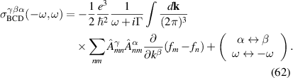
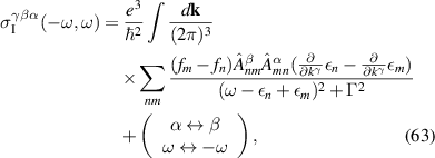
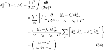
Appendix B.: Sum rule computations
The second order rectification conductivity in general is given by:

where J stands for 'Jerk', BCD for 'Berry curvature dipole', I for 'Injection' and S for 'shift current' respectively. We consider band structure with small relaxations (). Each contribution is given by:


For purposes of ensemble averaging over incoming random light, we need to consider only diagonal components of the nonlinear rectification conductivity, namely .

To simplify the notation for further analysis we write:
Thus, the conductivity which is the one that enters into the SRV, is:


TRS implies:


TRS makes the Jerk, Injection and the part proportional to of the Shift current vanish after momentum integration. Thus the contribution to the total rectification conductivity is given by BCD and resonant part of the shift current:
![$\mathrm{Re}\left[Q^{\gamma\alpha\alpha}\right]$](https://content.cld.iop.org/journals/0022-3727/54/40/404001/revision3/dac118fieqn53.gif)
In limit, we can simplify the expression using the following relation:

Now we can write a general version of the sum rule by including the spectral weight, which we assume to be a smooth function of ω, to obtain:
where and all zero-frequency contributions vanish under the assumption of absence of spectral weight ().


Now in the case of the operational definition of the BPRT, we consider the net change of the polarization coursed by pulse-like electric field:

In this set-up, without assuming TRS the resulting change of the polarization is:

where . As we see this result contains two extra terms proportional to 1/Γ which arise from the Jerk and injection current terms, but which vanish under the assumption of time-reversal symmetry.
Appendix C.: Computation details
The exchange and correlation energies were considered in the generalized gradient approximation with Perdew–Burke–Ernzerhof functional [36]. We projected the Bloch wave functions into high-symmetry atomic-orbital-like Wannier functions with diagonal position operator and considered all the electrons, which guarantees the full band overlap from ab-initio and Wannier functions in the energy window from −20 to 20 eV. The calculated band structures of TaAs and LiAsSe2 are shown in figure 5. Based on the highly symmetric Wannier functions, we constructed tight-binding (TB) model Hamiltonians and calculated the BCD and second order optical conductivity tensor. The γ (with α, β, γ = x, y, z) component of Berry curvature for the nth band at k point is computed by following:
where, is the Berry connection of nth band of Hamiltonian and is the Levi-Civita tensor. The BCD was calculated from the Berry curvature in a differential manner and with integral in the whole -space [17]:


where is the Berry curvature vector and fn is a Fermi–Dirac distribution. The relation between two and three index BCD tensors is:


Figure 5. Band structures of (a) TaAs and (b) LiAsSe2. Rectification conductivities of (c) TaAs and (d) LiAsSe2.
Download figure:
Standard image High-resolution imageThe second order optical conductivity tensor is calculated by the following expression:
here n
is nth band energy. The expression above is equivalent to expressions discussed in [5, 10] (see appendix D). The numerical results are consistent with the symmetry analysis. The plots showing the frequency dependence of the second order rectification conductivities of TaAs and LiAsSe2 are shown in figure 5. These plots show only the interband shift currents, since the BCD is simply a delta function peak at zero frequency.
After a k-grid convergency test, it was found that the change of BCD for TaAs is less than 5% with k-grid increasing from 360 × 360 × 360 to 480 × 480 × 480. A similar k-grid convergency was obtained with a k-grid of increasing from 240 × 240 × 240 to 360 × 360 × 360 for the second order optical conductivity in TaAs and LiAsSe2.
Appendix D.: Equivalence with other formalisms in the literature
Here we discuss the equivalence of our formulae for the rectification conductivity from equation (60) and others employed in the literature [1, 2, 4, 5, 9, 32, 39, 40]. Importantly, we show that shift currents derived in classic papers [1, 2] are only valid for Galilean systems, where spin orbit coupling is neglected, but not in general.
D.1. Comparison with [5, 39]
Here we will demonstrate that the interband rectification current in time reversal invariant materials arising from from equations (61)–(64), is identical to that from [5, 32]. This is the part of the rectification conductivity that controls the inter-band contribution to the QRSR and BPRT, but it is missing the intraband BCD contribution. This interband part however is the only one contributing to the SRV.

We define the following notation:


where and (a, b, c) are space indices. Alternatively, this can be written as:


where , and
By using the identity identity , one obtains:
![$[r^a,r^b] = 0$](https://content.cld.iop.org/journals/0022-3727/54/40/404001/revision3/dac118fieqn66.gif)

which leads to an alternative form to denote the generalized derivative:
for n ≠ m. By using equations (83) and (88) one can obtain that the conductivity from [5, 39] can be written as:

this is the same as the sum of the real part of injection and shift currents assuming time-reversal invariant conditions from equation (60), discussed in section (see appendix B), which were the ones employed in the main text. In the main text, we are also omitting the '0' in the conductivity arguments, but it is implicit every time we refer to a 'rectification' conductivity.

D.2. Comparison with [1, 2, 9]
We will here compare our formula from the current paper and [10] to the formulae from the classic [1, 2] (see e.g. [38, 40] for an application of this) and those of more recent work of [9] (see also [41–43] for closely related formulae to [9]). We will show that [1, 2] are missing crucial corrections that can only be neglected if one assumes the system to have an underlying parabolic dispersion (namely ignores spin–orbit coupling). On the other hand we will show that, upon proper regularization of infinitesimal imaginary parts in the frequency denominators, the formulae of [9] are equivalent to those we employ in the current paper and in our previous work [10].
Following [9] we write the second order perturbation to the Hamiltonian, as:


where is total Hamiltonian, is unperturbed band Hamiltonian, is electric field and


where means that one omits terms when denominator vanishes and latin sub-indices, (a, b, c) denote band labels, while upper greek indices (α, β, γ) denote space components.

From the above, the second order rectification conductivity is found to be:
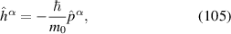
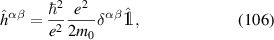
Here , with fa the Fermi–Dirac occupation of band a. We will compare the expression above with the expression from [1, 2]. [1, 2] employed the same gauge of [9], but assumed that the electrons have an underlying parabolic kinetic energy in addition to the periodic potential, and thus entirely neglects spin–orbit coupling effects. Therefore, the second order perturbed Hamiltonian for a single electron in [1, 2] has the form:


where m0 is the bare electron mass. The second order rectification conductivity of [1, 2] is therefore found to be:

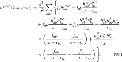
For purposes of comparing both expressions it is convenient to split them into pieces. The conductivity from [1, 2] we split as follows:

where KB stands for Kraut-Baltz from [1, 2]. We also split the conductivity from equation (95) [9] into the following terms:


where PM stands for Parker–Morimoto–Orenstein–Moore. Also we want to use one more index for each sub-term in these expressions. Namely, we will denote by the firs term from expression , and analogously for other terms.


By comparing equations (90), (91) and equations (96) and (97), we see that for systems considered in [1, 2] certain additional constrains are satisfied for the matrix elements as a consequence of the underlying parabolic dispersion. More specifically, the interband rectification conductivity from [1, 2], can be obtained from the formula of [9], upon enforcing the following relations:

From the expressions above one can see that the terms we have labeled PM0 and PM1 would vanish, because the tensor , is diagonal in the (a, b) band indices, and therefore its contribution to the rectification conductivity vanishes after multiplying by the difference of Fermi occupation functions, , which are only non-zero for a ≠ b. Now one can verify that the remaining terms agree between the two theories, specifically as follows:


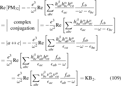
Expressions for and can be obtained from and respectively by swapping indices . Such a symmetrization automatically implied by conductivity once it is contracted with electric field indices, as is used for current expression in [2]. Thus we conclude the conductivity from [2] is equivalent to the sum of terms and .
![$\mathrm{Re}[\textrm{PM}]_{22}$](https://content.cld.iop.org/journals/0022-3727/54/40/404001/revision3/dac118fieqn77.gif)
![$\mathrm{Re}[\textrm{PM}]_{31}$](https://content.cld.iop.org/journals/0022-3727/54/40/404001/revision3/dac118fieqn78.gif)
![$\mathrm{Re}[\textrm{PM}]_{21}$](https://content.cld.iop.org/journals/0022-3727/54/40/404001/revision3/dac118fieqn79.gif)
![$\mathrm{Re}[\textrm{PM}]_{32}$](https://content.cld.iop.org/journals/0022-3727/54/40/404001/revision3/dac118fieqn80.gif)

![$\mathrm{Re}[\textrm{PM}]_{2}$](https://content.cld.iop.org/journals/0022-3727/54/40/404001/revision3/dac118fieqn82.gif)
![$\mathrm{Re}[\textrm{PM}]_{3}$](https://content.cld.iop.org/journals/0022-3727/54/40/404001/revision3/dac118fieqn83.gif)
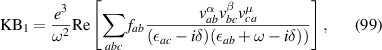
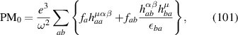
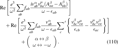
Note that in general (for example in the presence of spin–orbit coupling) and do contribute to the conductivity. These terms include not only intra-band terms, but also some contribution to interband shift currents terms that are missing in [1, 2], and are given by:
![$\mathrm{Re}[\textrm{PM}]_{0}$](https://content.cld.iop.org/journals/0022-3727/54/40/404001/revision3/dac118fieqn84.gif)
![$\mathrm{Re}[\textrm{PM}]_{1}$](https://content.cld.iop.org/journals/0022-3727/54/40/404001/revision3/dac118fieqn85.gif)
Or in notations used in [1, 2]:

To show that the extra shift current contribution, which we demonstrate above, is crucial—we will compute our Quantum Rectification Sum Rule for shift currents described in [1, 2] and [9]. With the proper regularization of the infinitesimal imaginary parts of the frequency denominators of both of these references, the frequency integration of interband conductivities are:

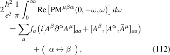
Therefore we see that while the expression for interband contribution to the sum rule obtained from [9] (equation (112)) is the same as the one derived in our previous paper [10], the one that would be derived from [1, 2] (equation (113)) differs from them. As previously discussed, this is because [1, 2] are missing some terms which only vanish if one assumes a parabolic dispersion which completely neglects the spin–orbit coupling.