


Abstract
Hot Neptunes are extrasolar planets that are similar in size to Neptune in our solar system but are much closer to their host stars, completing an orbit in 10 days or less. The origin of hot Neptunes is not fully understood. A potential large third body at a distance can lead to the migration of long-period planets to become much closer to the host star, and such a dynamical process helps explain the origin of hot Jupiters. We investigate whether hot Neptunes could share a similar origin by analyzing radial velocity data from multiple sources for a sample of 34 hot Neptune systems. Hot Neptune systems appear to have similar values of linear trend to hot Jupiter systems. We perform a maximum likelihood analysis to constrain the mass and distance distribution of the putative third body. The overall fraction of hot Neptune systems with third bodies is consistent with unity, higher than 71% at the 2σ level. On average, the mass and distance distribution of the third bodies for hot Neptune systems is consistent with that for hot Jupiter systems. Our results suggest that hot-Neptune systems share the same origin mechanism as hot Jupiters, e.g., through the gravitational effect of third bodies.

Original content from this work may be used under the terms of the Creative Commons Attribution 4.0 licence. Any further distribution of this work must maintain attribution to the author(s) and the title of the work, journal citation and DOI.
1. Introduction
Observations of extrasolar planets have revealed a variety of populations and enabled statistical studies to learn about their formation and evolution (e.g., Zhu & Dong 2021). Hot Neptunes are extrasolar planets that are similar in size (about 2–6 Earth radii) to Neptune in our solar system but are much closer to their stars, completing an orbit in 10 days or less (Dong et al. 2018), in comparison to 165 yr for our Neptune. The origin of hot Neptunes is not fully understood. In this work, we aim to investigate the origins of hot Neptunes based on radial velocity (RV) data.
Hot Neptunes share remarkable similarities with hot Jupiters (Dong et al. 2018). Both populations more likely reside in metal-rich stars and in systems with single-transiting planets. Furthermore, the dependence of their frequencies on host metallicity is similar, increasing by a factor of approximately 10 from subsolar to supersolar metallicity regimes. For each metallicity subsample, the frequencies of hot Neptunes and hot Jupiters are similar within a factor of 2. On the origin of hot Jupiters (see a review by Dawson & Johnson 2018), one theory suggests that the gravity of a massive third outer body brings a long-period Jupiter onto an orbit of high eccentricity (e.g., through the Lidov-Kozai mechanism; Lidov 1962; Kozai 1962 ) and the subsequent tidal dissipation leads to an orbit much closer to the star.
The first-order effect caused by the acceleration induced by the gravity of the putative third body would show up as a linear trend in the long-term RV variation of the planet system. Studying the linear trend in RV data of hot-Jupiter systems (e.g., Knutson et al. 2014) and searching for long-period companions (e.g., Bryan et al. 2016) lend support to the above dynamical origin mechanism for hot Jupiters.
Given the similarities between hot Jupiters and hot Neptunes mentioned above, it is natural to ask whether the same dynamical process can also explain the origin of hot Neptunes. The accumulated RV observations over the past decades (e.g., Trifonov et al. 2020) for hot-Neptune systems have made such an investigation possible.
In this work, we analyze the RV data for a sample of hot Neptunes, aiming to shed light on the origins of such a population of exoplanets. We present the sample of hot-Neptune systems, the RV data, and the method in Section 2. In Section 3, based on modeling the RV data, we compare the linear trend distributions of hot-Neptune and hot-Jupiter systems and constrain the distribution of the potential third bodies. We summarize and discuss our results in Section 4.
2. Data and Method
We construct a sample of hot-Neptune systems based on the NASA Exoplanet Archive. 1
We apply various filters by defining hot Neptunes to have orbital periods of 10 days or less and sizes of 2–6 Earth radii, and by requiring that they were discovered through the transit method. In total, 580 exoplanets are identified. The period and radius distribution of these selected extrasolar planets are shown as blue points in Figure 1.

Figure 1. Distribution of hot Neptunes as a function of orbital period and planet radius. The blue dots represent all the hot Neptunes selected from the Exoplanet Archive, while the red dots represent those with enough RV data for our study, which form the sample of hot-Neptune systems in this work.
Download figure:
Standard image High-resolution imageNext, to constrain the linear trends, the selected systems need to have RV observations. The HARPS RV Bank (Trifonov et al. 2020) provides convenient RV data, with precise measurements from a uniform and improved spectroscopic pipeline. We use the HARPS RV Bank as our initial source of RV data. We search the HARPS RV Bank (Trifonov et al. 2020) and keep only those systems that have RV data in the Bank. We end up with 34 hot-Neptune systems for our investigation, which are marked as red points in Figure 1. Among them, 12 (22) appear to be single-planet (multiplanet) systems. For each system, in order to better constrain the RV trend, we further supplement the RV data with those found in literature (as listed in Table 1).
Table 1. Linear Trend Constraints from Our Model Fitting to the RV Data of Hot-Neptune Systems
| Name | Linear Trend | Nplanet | RV Data Sources |
|---|---|---|---|
| (10−2 ms−1d−1) | |||
| CoRoT-7 | 24.851 ± 4.414 | 3 | (1, 8) |
| CoRoT-22 | 0.766 ± 0.598 | 1 | (1, 2) |
| CoRoT-24 | −3.119 ± 0.733 | 2 | (1, 5) |
| GJ163 | −0.042 ± 0.044 | 5 | (1, 18) |
| GJ433 | 0.448 ± 0.416 | 3 | (1) |
| GJ480 | −0.607 ± 0.337 | 1 | (1) |
| GJ436 | −0.103 ± 0.057 | 1 | (1) |
| GJ536 | −0.065 ± 0.021 | 1 | (1) |
| GJ581 | 0.016 ± 0.019 | 3 | (1) |
| GJ674 | 0.031 ± 0.014 | 1 | (1) |
| GJ876 | 1.077 ± 0.400 | 4 | (1, 19) |
| GJ1214 | 3.732 ± 18.410 | 1 | (1, 12) |
| GJ1265 | −0.034 ± 0.039 | 1 | (1, 15) |
| GJ3470 | −0.134 ± 0.137 | 1 | (1, 21) |
| GJ3634 | 2.497 ± 0.078 | 1 | (1) |
| GJ9827 | −2.091 ± 1.204 | 3 | (1, 22 ) |
| HD1461 | −0.085 ± 0.010 | 2 | (1, 10, 11) |
| HD10180 | 0.032 ± 0.012 | 6 | (1) |
| HD39091 | −0.034 ± 0.024 | 3 | (1, 4) |
| HD47186 | 0.472 ± 0.025 | 2 | (1, 7) |
| HD77338 | −0.075 ± 0.033 | 1 | (1, 9) |
| HD96700 | −0.028 ± 0.011 | 3 | (1) |
| HD106315 | 0.093 ± 0.114 | 2 | (1, 3) |
| HD109271 | −0.095 ± 0.041 | 2 | (1, 6) |
| HD134060 | −0.020 ± 0.015 | 2 | (1) |
| HD176986 | 0.015 ± 0.030 | 2 | (1) |
| HD181433 | 0.391 ± 0.039 | 3 | (1, 16) |
| HD215497 | −0.026 ± 0.068 | 2 | (1) |
| HD219828 | −0.013 ± 0.035 | 2 | (1, 23) |
| HD285968 | −0.257 ± 0.080 | 1 | (1, 25) |
| HIP54373 | −0.085 ± 0.072 | 2 | (1, 14) |
| K2-27 | −1.042 ± 0.501 | 1 | (1, 20) |
| K2-32 | 0.075 ± 0.116 | 4 | (1, 24) |
| K2-138 | 10.027 ± 2.417 | 6 | (1, 17) |
Note. reference list: (1) Trifonov et al. (2020); (2) Moutou et al. (2014); (3) Kosiarek et al. (2020); (4) Gandolfi et al. (2018); (5) Alonso et al. (2014); (6) Santos et al. (2016); (7) Bouchy et al. (2009); (8) Haywood et al. (2014); (9) Jenkins et al. (2013); (10) Rivera et al. (2009); (11) Rosenthal et al. (2021); (12) Anglada-Escudé et al. (2013); (13) Feng et al. (2019); (14) Luque et al. (2018); (15) Horner et al. (2019); (16) Lopez et al. (2019); (17) Bonfils et al. (2013); (18) Laughlin et al. (2005); (19) Petigura et al. (2017); (20) Bonfils et al. (2012); (21) Teske et al. (2018); (22) Santos et al. (2016); (23) Lillo-Box et al. (2020); (24) Butler et al. (2009).
Download table as: ASCIITypeset image
For the sample of the 34 hot-Neptune systems, their properties are similar to those of the parent sample. For example, the mean and standard deviation of the periods of the parent sample and selected sample are 6.0 ± 2.3 days and 5.9 ± 2.4 days, respectively. For radius, they are 2.9 ± 0.8 and 3.3 ± 1.0 earth radii; and for host star metallicity, 0.02 ± 0.16 and 0.07 ± 0.17.
We use exostriker (Trifonov 2019) to model the available RV data for each system in our sample and constrain the orbital parameters (e.g., period, semimajor axis, and eccentricity) of its planets and the linear trend. The initial inputs about planets' orbits are based on values found in literature. 2 In particular, the number of planets and the orbit period of each planet are our adopted prior in performing the modeling. The jitter term is included in the error budget to ensure that the best fit has a reduced χ2 value of unity. We find that the jitter values range from 0 to 50 m s−1, in broad agreement with those found in stellar jitter studies (e.g., Bastien et al. 2014) and in hot-Jupiter studies (e.g., Knutson et al. 2014).
As an example, in Figure 2, we show the RV observation and the model fit for HD285968. The band in the left panel is in fact the sine-like curve with a period of 8.77 days from the model. When folded with the hot Neptune's orbital period of 8.77 days, the RV variation of the host star as a function of the phase can be seen in the right panel. In the left panel, the RV fit shows a clear slope. With RV data covering a baseline of ∼10 yr, the linear trend for this system is detected with high significance, (−2.57 ± 0.80) × 10−3 ms−1d−1.

Figure 2. RV measurements and model of HD285968. Left: two sets of RV observations (blue and red data points, respectively) with the best-fit model (gray), and the bottom panel shows the residual from the model fit. A significant linear trend is detected for this system. Right: RV data (with linear trend removed) folded into the planet's orbital period, and the bottom panel shows the residual from the model fit with the gray band indicating the mean jitter value.
Download figure:
Standard image High-resolution imageIn the example shown in Figure 2, there are two sets of data (represented by blue and red points) with a clear RV offset. Between the ∼2552 day gap, an upgrade of the optical fibers for HARPS occurred in 2015 May (Trifonov et al. 2020). It may raise the question of whether the linear trend is an artifact caused by the instrument systematics in the RV measurements. However, this does not appear to be the case. First, the relative offset of the two sets of data has been accounted for in the model fitting, since it is included as a free parameter. Additionally, the model parameters (including the linear trend) remain consistent when fitting the first set of data (blue) alone. The second data set (red) has a shorter baseline, leading to weaker model constraints, but they are again consistent with those from fitting both data sets.
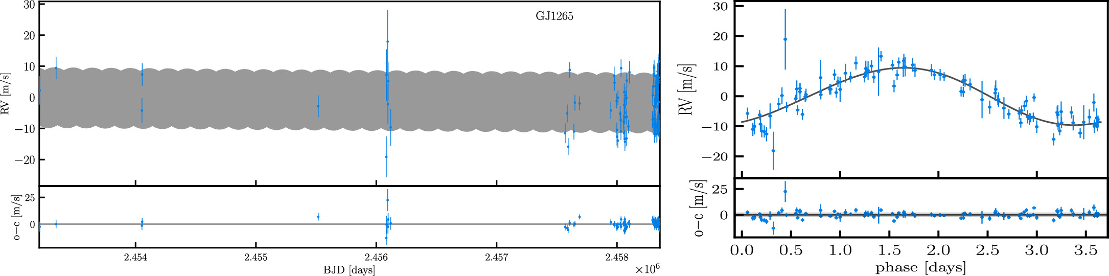
Figure 3 shows the RV fitting results for GJ1265, with observational data also covering a baseline of about 10 yr. This system is posed as an example of no significant detection of the linear trend, (−3.4 ± 3.9) × 10−4 ms−1d−1.

Figure 3. Similar to Figure 2, but for GJ1265. No significant linear trend is detected for this system.
Download figure:
Standard image High-resolution imageHD1461 is a system with two known planets, and its RV fitting results are plotted in Figure 4. From the RV data, the effect of the two planets, with one being the hot Neptune, clearly shows up. With observation covering a baseline of ∼5000 days, the quadratic trend in the RV data is detected.

Figure 4. Similar to Figure 2, but for HD1461, which has a significant quadratic trend detected and has two planets.
Download figure:
Standard image High-resolution imageIn Table 1, the linear trend constraints for the 34 hot-Neptune systems are listed. To derive the constraints, the model only includes RV trend to the linear order. We then extend the model to have both linear and quadratic terms in the RV trend. Table 2 lists the RV trend constraints for systems with significant quadratic term.
Table 2. RV Trend Constraints for Systems with Significant Quadratic Trend
| Name | Linear Trend | Quadratic Trend |
|---|---|---|
| (ms−1d−1) | (ms−1d−2) | |
| CoRoT-24 | (−1.04 ± 0.18) × 10−1 | (5.95 ± 1.51) × 10−5 |
| HD1461 | (−2.83 ± 0.33) × 10−3 | (5.0 ± 0.8) × 10−7 |
| HD176986 | (4.96 ± 0.87) × 10−3 | (−1.04 ± 0.17) × 10−6 |
| HD181433 | (1.90 ± 0.11) × 10−2 | (−3.76 ± 0.27) × 10−6 |
Download table as: ASCIITypeset image
3. Constraints on the Linear Trends and the Third-body Distribution
We first analyze the derived linear trend constraints for our sample of hot-Neptune systems and compare them with those for hot-Jupiter systems. Then, we perform further analysis of the RV data to study the implications for the distributions of masses and distances of the perturbing objects and make comparisons to those for hot-Jupiter systems.
With our hot-Neptune systems, we test for correlation between the absolute value of the linear trend and planet parameters, including planet radius, orbit period, and orbit eccentricity. We find no clear dependence of the linear trend constraints on these planet parameters.
Among the 34 hot-Neptune systems, six systems have linear trend detection. In addition, four systems have quadratic trend detection. These numbers are 12 and 3 for the hot-Jupiter systems. The overall fraction of hot-Neptune systems with acceleration detection (10 out of 34) is similar to that of hot-Jupiter systems (15 out of 51).
In the top panel of Figure 5, we show the linear trend constraints as a function of planet mass for hot-Neptune systems from this work and for hot-Jupiter systems in Knutson et al. (2014). The sign of the linear trend is of no importance for our discussion and is neglected. For consistency, four hot-Neptune systems with significant quadratic trends and three hot-Jupiter systems with clear curvature in the fits are not shown. Filled circles with error bars represent systems with significant (>3σ) linear trend detection, while open circles show those without 3σ detection.

Figure 5. Comparison of linear trends for systems with hot Neptunes (blue) and hot Jupiters (red). The results for hot Neptunes are from this work and those for hot Jupiters are taken from Knutson et al. (2014). Filled and open circles are for systems with and without significant (>3σ) linear trend detection. The top and bottom panels correspond to analysis of hot-Neptune systems with the original RV data and with the shorter baseline data, respectively. See the text for detail.
Download figure:
Standard image High-resolution imageThe distributions of linear trends of hot-Neptune and hot-Jupiter systems appear to be different, if we treat the best-fit values plus and minus error bars as the whole constraints. For hot-Jupiter systems, the linear trend constraints are clustered around a few times 10−2ms−1d−1. While some hot-Neptune systems have linear trend constraints at such a level, a large faction of them have linear trends about more than one order of magnitude lower, down to a few times 10−4ms−1d−1.
The linear trend constraints depend on the baseline of observation. Since constraints on hot-Jupiter systems used in the comparison typically have shorter baselines than hot-Neptune systems in this work, for fair comparison, we perform a test by using shorter baselines for hot-Neptune systems. We take the average baseline (∼1900 days) for hot-Jupiter systems. For hot-Neptune systems with observation baseline shorter than 1900 days, we keep all the RV data, while for those with baseline longer than 1900 days, we only keep the observed data up to the first 1900 days. With the shorter-baseline data, we redo the model fits to obtain constraints. The number of systems with significant acceleration detection becomes seven (five with linear trend detection and two with quadratic trend detection). The linear trend constraints from the shorter baseline data are shown in the bottom panel of Figure 5. While the uncertainties in the constraints become larger, they are on average still smaller than those for hot-Jupiter systems, indicating the contribution of factors like signal-to-noise of the data to the constraints. While the overall trend in the bottom panel is similar to that in the top panel, it becomes less different from the hot-Jupiter constraints (especially when those with significant detections are compared).
To put the linear trend values into context, we can express the expected linear trend caused by a third body of mass m at distance a from the system as
or

where θ is the angle between the line of sight and the line connecting the star and the third body.
The linear trend constraints, if taken at face values, seem to hint that the third bodies for hot-Neptune systems on average have lower mass and/or are farther from the host stars. The six hot-Jupiter systems with their hot-Jupiter mass starting to overlap with hot-Neptune masses (≲0.3MJ ) seem to follow the linear trend constraints seen in the hot-Neptune systems. However, if we focus on those with significant detections, linear trends for hot-Neptune systems and hot-Jupiter systems do not differ substantially. In what follows, we perform more quantitative comparisons based on Kolmogorov–Smirnov tests and maximum likelihood analysis.
3.1. Linear Trend Comparisons from Kolmogorov–Smirnov Tests
To quantify the potential difference in the distributions of RV linear trend, we perform the Kolmogorov–Smirnov (KS) tests.
For many systems, we only have loose linear trend constraints, with no significant detection. The uncertainties in the constraints are typically larger for the hot-Jupiter systems. As an attempt to account for the full range of linear trend constraints, for each system we sample the full distribution, assumed to be a Gaussian distribution centered at the best-fit linear trend value with the standard deviation being the 1σ error bar of the constraints. In detail, the linear trend of each system is represented by 10,000 sampled values. We then compare the cumulative distribution functions (CDFs) of the sampled values for all hot-Neptune systems and hot-Jupiter systems and derive the maximum difference between the CDFs and the corresponding p value. The linear trend constraints of hot-Neptune systems appear to peak at lower values than those of hot-Jupiter systems. The p value is about 0.033%. With constraints from shorter baseline data for hot-Neptune systems, the p value is about 0.11%.
While the above p values may signal a difference, they are not necessarily as meaningful as those from the situation that all systems have stringent linear trend constraints. A more appropriate KS test is to limit the comparison to systems with significant linear trend detections. Taking the best-fit linear trend values for hot-Neptune and hot-Jupiter systems with significant linear trend detection, we find a p value of 0.25. If we repeat the test with the shorter baseline results for hot-Neptune systems, the p value changes to 0.40. These p values indicate no significant difference.
Given that a large fraction of hot-Neptune and hot-Jupiter systems have no significant linear trend detection, the KS tests only serve as a preliminary comparison to provide a crude evaluation of the difference in the linear trend constraints. The above tests suggest that the difference between the linear trend constraints for hot-Neptune and hot-Jupiter systems, if it exists, may not be clearly revealed by the KS tests with the data sets we use for the comparison. To fully account for the uncertainties in the constraints and the effect of the putative third bodies, we turn to a maximum likelihood analysis.
3.2. Maximum Likelihood Analysis of the Third-body Distribution
To fully account for the cases of both detections and nondetections of linear RV trend, we implement a maximum likelihood method to constrain the mass and distance distributions of the potential third body and compare the results for hot-Neptune and hot-Jupiter systems.
As the first step, for each hot-Neptune system, we add a putative third body to fit the RV data (Wright et al. 2007), together with the existing planet(s). For the i-th hot-Neptune system, we find the best-fit χ2 value, , at each location on a grid of semimajor axis a and third-body mass (assuming zero eccentricity; for simplicity, hereafter we use m for ). Similar to Knutson et al. (2014), we set the range of m to be 0.2–500MJ and that of a to be 1–100 au. The likelihood for the third body to have the corresponding m and a is computed as


where is the minimum of all the values.


The results of the constraints on the mass and distance of the putative third body (a.k.a. Wright plots) for all the systems are shown in the Appendix (Figure 17). Figure 6 shows two examples. In the first example (GJ876; left panel), the combination of mass and distance is constrained. The third body can be a low-mass one closer to the star or a high-mass one farther away from the star. This is largely driven by the fact that the linear trend is proportional to m/a2, as shown in Equations (1) and (2), and the RV data does not show significant trend beyond the linear order. For comparison, the RV data for the system CoRoT-24 show significant quadratic trend (see Figure 14 in Appendix A), allowing good constraints on the mass and distance of the third body (∼2MJ at ∼4 au).

Figure 6. Two examples of constraints on the mass and distance of the putative third body. While for the hot-Neptune system in the left panel, the combination of mass and distance of the third body is constrained, for the one in the right panel, the mass and distance of the third body are well-constrained. The contours correspond to the 1σ, 2σ, and 3σ confidence levels, respectively.
Download figure:
Standard image High-resolution imageWith the third body's mass and distance constraints for each hot-Neptune system, we perform the maximum likelihood analysis to obtain the constraints on the mass and distance distribution of the third body. Following previous work (e.g., Tabachnik & Tremaine 2002; Knutson et al. 2014), we model both the mass (m) and the distance (a) distribution as power law,

where C is the normalization factor. Instead of leaving C as a free parameter (e.g., Knutson et al. 2014), we fix it for given values of α and β by requiring . We then introduce a fraction parameter F to explicitly incorporate the possibility that only a fraction of the systems have a third body. The third-body distribution is then described as f(m, a) = F × Cmα aβ . By definition, F is the fraction of systems with third bodies and has values between 0 and 1. We consider three sets of hot-Neptune systems: the whole sample, the sample of single-planet systems, and the sample of multiplanet systems. For each set of samples, we aim to constrain α, β, and F. Comparisons of the constraints for different samples allow us to tell how different their third body distributions are.
Given the observational data, for each distribution model represented by the model parameters (α, β, F), the probability to have a detection for system i is computed as

where pi (m, a) is the probability in the corresponding (, ) cell in the normalized Wright plot, derived based on Equation (3). The probability of nondetection is then . The total likelihood of the model for a given sample is (Tabachnik & Tremaine 2002; Knutson et al. 2014)


where Nd is the number of systems with a significant (>3σ) linear trend detection and Nnd is that for nondetection.
We apply the maximum likelihood analysis to all the hot-Neptune systems. Figure 7 shows the marginalized distribution in the α–F and β–F plane. The parameter F, representing the overall fraction of systems with third bodies, is consistent with unity. In fact, the maximum likelihood occurs at F = 1, with α = − 0.253 and β = 0.114. The marginalized distribution of F peaks at F = 1, and we find F > 0.88, >0.71, and >0.52 at the 68.3%, 95.4%, and 99.7% confidence level.

Figure 7. Marginalized distributions of the third body mass and distance distribution parameters in the α–F (top) and β–F (bottom) plane. The parameter F is the overall fraction of hot-Neptune systems with third bodies, and α (β) is the power-law index of the mass (distance) distribution function. The contours in each panel correspond to 1σ, 2σ, and 3σ confidence levels.
Download figure:
Standard image High-resolution imageThe marginalized distribution of model parameters α and β constrained from all the hot-Neptune systems is shown in the left panel of Figure 8 (blue shaded contours). We find that the contours do not vary much if F is fixed to unity. The 1σ, 2σ, and 3σ constraints for α are (−0.59, −0.17), (−0.84, 0.01), and (−1.14, 0.19), respectively. Those for β are (−0.20, 0.39), (−0.50, 0.72), and (−0.80, 1.10).

Figure 8. Constraints on the third-body mass and distance distribution parameters α and β. The parameter α (β) is the power-law index of the mass (distance) distribution function. The blue shaded contours are constraints for all hot-Neptune systems, while the cyan and black dashed contours are for single- and multiplanet hot-Neptune systems. For comparison, the constraints of the third-body distribution for hot-Jupiter systems (red; adopted from Knutson et al. 2014) are overlaid. The contours correspond to 1σ, 2σ, and 3σ confidence levels for two parameters, respectively. The left, middle, and right panels correspond to analysis of hot-Neptune systems with the original RV data, with the shorter baseline data, and with the original data by applying weights, respectively. See the text for detail.
Download figure:
Standard image High-resolution imageIf the hot-Neptune systems are divided into those of single- and multiplanet systems, the constraints on the model parameters appear to be consistent with each other (see the black and cyan dashed contours).
As a comparison, in the left panel of Figure 8 we also show the constraints on the third-body distribution for hot-Jupiter systems (red dashed contours; adopted from Knutson et al. 2014). The 1σ contours for hot-Neptune and hot-Jupiter systems are well separated. For parameter α, the 2σ ranges of the marginalized distributions for the hot-Neptune and hot-Jupiter systems are different, (−0.84, 0.01) versus (0.1, 2.3). The lower values of α for hot-Neptune systems suggest that the corresponding third bodies on average tend to have lower masses. For parameter β, the hot-Neptune systems have slightly lower values, indicating third bodies closer to the host stars. However, the constraints for β are mostly consistent with those from hot-Jupiter systems, e.g., with 1σ ranges of (−0.20, 0.39) versus (0.3, 1.0). As a whole, the third-body distributions for hot-Neptune and hot-Jupiter systems are consistent with each other (e.g., with 2σ contours overlapped), showing no significant differences.
In the middle panel of Figure 8, we show the comparison based on the analysis using the shorter baseline data for hot-Neptune systems. As expected, the constraints become loosened, and the difference from the hot-Jupiter results becomes even less significant.
Finally, as a test, in the right panel of Figure 8, we show the results based on an maximum likelihood analysis with weight assigned to each hot-Neptune system. The motivation is to approximately test how the constraints may change if the whole parent sample (blue points in Figure 1) is uniformly sampled. We divide the period-radius plane into 17 rectangular cells, with each cell including at least one hot-Neptune system in our sample (red points in Figure 1). We assign weight to each hot-Neptune system in our sample as the ratio of the number of blue points to that of red points in the corresponding cell and perform the maximum likelihood analysis. The resulting contours shift. For example, the contours from all hot-Neptune systems shift toward lower α and higher β. However, the constraints remain consistent with the original constraints in the left panel. They also remain consistent with the hot-Jupiter results.
Overall, while the results from the maximum likelihood analysis qualitatively agree with those indicated by the linear trend distributions and those from the KS tests, they clearly show that the difference in the third-body distributions for hot-Neptune and hot-Jupiter systems is not significant. Both the linear trend comparison and the KS tests have the degeneracy between mass and distance of the third body (e.g., Equation (1)). The maximum likelihood analysis helps break such a degeneracy, as the RV data can provide constraints on the orbital motion of the putative third body.
4. Summary and Discussion
We analyze the acceleration trends in the RV data of hot-Neptune systems and compare their distribution to that of hot-Jupiter systems, in order to test the theory about the origin of the hot-Neptune systems under the gravitational influence of a third body.
For our hot-Neptune systems, approximately 29% (10/34) have a significant linear trend or quadratic trend, similar to the proportion in hot-Jupiter systems (15/51≃29%). For single-planet hot-Neptune systems, this number is 25% (3/12). The results strongly indicate the existence of external third bodies, supporting the dynamic origins of hot Neptunes.
In detail, the linear trend distribution simply based on the constraints for all the hot-Neptune systems and that for the hot-Jupiter systems appear to be different, with the former having more systems with lower linear trends. However, the significance of the difference cannot be readily told, as the constraints depends on observation baseline and many systems do not have linear trend detection. If we limit to systems with significant linear trend, based on KS tests, we find no evidence for difference in the linear trend distribution between hot-Neptune and hot-Jupiter systems. To fully account for acceleration trend constraints, we employ a maximum likelihood analysis to constrain the mass and distance distribution of the putative third body.
The maximum likelihood analysis of the mass and distance distribution of the external third bodies shows that the overall fraction of hot-Neptune systems with third bodies is consistent with unity, higher than 71% at a 2σ confidence level. On average, the external bodies for hot-Neptune systems are lower in mass than those for hot-Jupiter systems, but the difference is only at the 2σ level. The third bodies for hot-Neptune systems also appear to be closer to host stars than those of hot-Jupiter systems, but again the difference is not significant. In the α–β plane, the 2σ contours for hot-Neptune and hot-Jupiter systems overlap, suggesting that no significant difference is found in the distribution of third bodies.
The constraints suggest that Neptune-like planets, being less massive than Jupiter-like planets, can be affected by external bodies similar to those for hot-Jupiter systems to migrate to become hot Neptunes.
The constraints on mass and distance of the third bodies of individual hot-Neptune systems in this work can guide the search for them, e.g., through imaging observations with adaptive optics (e.g., Bryan et al. 2016). For example, nine of the hot-Neptune systems (CoRoT-24, GJ480, GJ536, HD1461, HD39091, HD77338, HD181433, HD285968, and K2-27) are interesting targets for observation, as the distance and mass of the putative third body have been tightly constrained from the RV analysis (see Figure 17). The observational search for third bodies would provide strong tests on the dynamic origins of hot Neptunes.
With RV observations of more hot-Neptune/Jupiter systems and in a longer time span, the constraints on the third bodies are expected to become tighter, which will help further test the origins of these extrasolar planet populations.
Acknowledgments
S.Z. thanks Subo Dong for his helpful guidance and insightful discussions. S.Z. also thanks the referee for their comments that helped improve the paper.
This research has made use of the NASA Exoplanet Archive, which is operated by the California Institute of Technology, under contract with the National Aeronautics and Space Administration under the Exoplanet Exploration Program.
Facility: Exoplanet Archive - .
Software: exostriker (Trifonov 2019).
Appendix A: RV Modeling for Systems with Significant Linear or Quadratic Trend Detection
Model fits to the RV data and the corresponding planet phase plots for two hot-Neptune systems with significant acceleration detection are shown in the main text (Figures 2 and 4). For completeness, we show in this appendix those for the other eight hot-Neptune systems with significant acceleration detection, five with significant linear trend detection (Figures 9–13), and three with significant quadratic trend detection (Figures 14–16).

Figure 9. Same as Figure 2, but for CoRoT-7, a hot-Neptune system with a significant linear trend detection.
Download figure:
Standard image High-resolution image
Figure 10. Same as Figure 2, but for GJ3634, a hot-Neptune system with a significant linear trend detection
Download figure:
Standard image High-resolution image
Figure 11. Same as Figure 2, but for GJ536, a hot-Neptune system with a significant linear trend detection.
Download figure:
Standard image High-resolution imageA few systems are worth mentioning. HD47186 has a significant linear trend detection (∼19σ; see Table 1). However, the model fit to its RV data (Figure 12) shows clear residuals. If we add quadratic term when fitting the RV data, the detection on the quadratic trend is barely significant (∼2.96σ). Therefore we formally put this system into the category of having a significant linear trend detection. More accurately, such residuals are a manifestation of a third body at work that will be characterized in our maximum likelihood analysis (Figure 17).

Figure 12. Same as Figure 2, but for HD47186, a hot-Neptune system with a significant linear trend detection.
Download figure:
Standard image High-resolution imageK2-138 has as many as six planets (Figure 13). Although the RV data only span about 70 days, given the period priors we adopt for the six known planets, the fit is able to show the effects of the six planets in the folded RV data.

Figure 13. Same as Figure 2, but for K2-138, a hot-Neptune system with a significant linear trend detection.
Download figure:
Standard image High-resolution imageFor CoRoT-24 (Figure 14), although we use the period priors for the two known planets, the phase-folded RV data do not show clear trends because of the large uncertainties in the data. The quadratic trend in the RV data, however, is strong enough to be detected, leading to good constraints on the mass and distance of the putative third body (right panel of Figure 6).
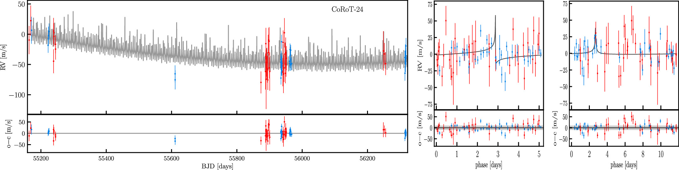
Figure 14. Same as Figure 4, but for CoRoT-24, a hot-Neptune system with a significant quadratic trend detection.
Download figure:
Standard image High-resolution image
Figure 15. Same as Figure 4, but for HD176986, a hot-Neptune system with a significant quadratic trend detection.
Download figure:
Standard image High-resolution image
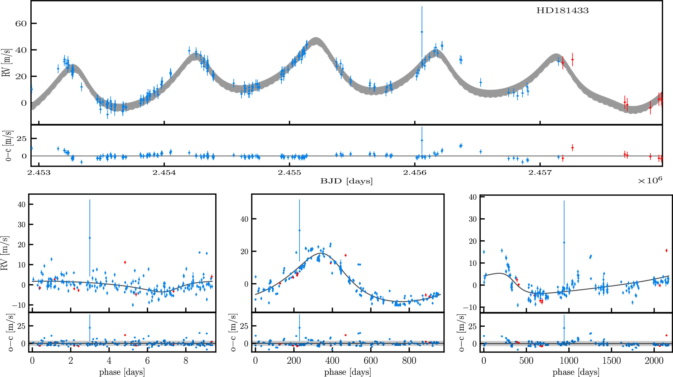
Figure 16. Same as Figure 4, but for HD181433, a hot-Neptune system with a significant quadratic trend detection.
Download figure:
Standard image High-resolution imageAppendix B: Constraints on the Third-body Distribution for Each Hot-Neptune System
For each hot-Neptune system, we fit the RV data by adding a putative body and obtain the constraints on the mass m and distance a (semimajor axis) of the third body (Wright et al. 2007). The results are shown in Figure 17, which are used in our maximum likelihood analysis. The contours correspond to Δχ2 = 2.30, 6.17, and 11.80, to approximate the 1σ, 2σ, and 3σ confidence levels for two parameters.

Figure 17. Constraints on the mass and distance distribution of the third body for each hot-Neptune system, obtained by adding a putative third body in fitting the RV data. The contours correspond to the 1σ, 2σ, and 3σ confidence levels for two parameters. No converged results are found for CoRoT-7 and GJ9827, and the corresponding panels are put as place holders. See text for more details.
Download figure:
Standard image High-resolution image
For CoRoT-7 and GJ9827, the fits do not converge at a large fraction of grid points. These two systems are excluded in our maximum likelihood analysis, although they are put as place holders in Figure 17.
The constraints in most systems show the expected trend of a larger mass at a larger distance. The RV data of several systems allow tighter constraints on the distribution of the third body. For the five systems with a significant quadratic trend detection, three of them (CoRoT-24, HD1461, and HD181433) have good constraints on the mass and distance of the third body. For systems with good linear trend constraints (≳2σ), some have good third-body distribution constraints, such as GJ536, HD77338, and HD285968, while GJ3634 and HD47186 show tight constraints along the m/a2 degeneracy direction.
Footnotes
- 1
- 2
Taken from http://www.exoplanet.eu/.