


Abstract
We present a systematic study of particle transport by diffusion in young pulsar wind nebulae (PWNe). We selected nine bright sources that are well resolved with the Chandra X-ray Observatory. We analyzed archival data to obtain their radial profiles of photon index (Γ) and surface brightness (Σ) in a consistent way. These profiles were then fit with a pure diffusion model that was tested on Crab, 3C 58, and G21.5−0.9 before. In addition to the spectral softening due to the diffusion, we calculated the synchrotron power and built up the theoretical surface brightness profile. For each source, we performed separate fits to the Γ and Σ profiles. We found that these two profiles of most PWNe are similar, except for Crab and Vela. Both profiles can be well described by our model, suggesting that diffusion dominates the particle transport in most sampled PWNe. The discrepancy of parameters between the Γ and Σ profiles is relatively large for 3C 58 and G54.1+0.3. This difference could be attributed to the elongated shape, reflecting boundary, and the nonuniform magnetic field. Finally, we found no significant correlations between diffusion parameters and physical parameters of PWNe and pulsars.

Original content from this work may be used under the terms of the Creative Commons Attribution 4.0 licence. Any further distribution of this work must maintain attribution to the author(s) and the title of the work, journal citation and DOI.
1. Introduction
An isolated pulsar releases most of its rotational energy through high-energy relativistic particle outflow called pulsar wind. When the pulsar wind interacts with the surrounding medium and is overpressured, a pulsar wind nebula (PWN) is formed. This drives a wind-termination shock, at which the particles are heated and reaccelerated to the ultrarelativistic regime (see reviews by Gaensler & Slane 2006; Slane 2017, p. 2159). The shocked particles move through the magnetic field in a PWN. They cool down and emit synchrotron radiation from radio to X-rays and inverse-Compton radiation in γ-rays.
Observationally, the injected particle distribution could be inferred from the broadband spectral energy distribution of PWNe. A one-zone model without spatial information can reproduce the observed properties (see, e.g., Pacini & Salvati 1973; Tanaka & Takahara 2010; Bucciantini et al. 2011; Vorster et al. 2013). The improvement of spatial resolution of instruments makes it possible to investigate the detailed structure and the evolution of PWNe. When transporting outward, the high-energy particles lose their energies on a fast timescale and result in a softening of the X-ray spectrum. At the same time, the synchrotron flux decreases. The radial profiles in the radio band have been first modeled as a diffusion nebula with a particle source injected at the center (Gratton 1972; Wilson 1972). A one-dimensional magnetohydrodynamic (MHD) model with a time-independent steady flow has been established from this idea and tested on Crab (Kennel & Coroniti 1984a, 1984b; Porth et al. 2014, 2016).
However, this model is not applicable for a few other PWNe under the unprecedented spatial resolution of Chandra X-ray Observatory (see, e.g., Slane et al. 2004). Combining the photon index (Γ) profile and the surface brightness (Σ) profile, Ishizaki et al. (2017) found that the simple MHD model with steady stream fails to reproduce observed properties in 3C 58 and G21.5−0.9, indicating that spatial diffusion of particles, which has been modeled by Tang & Chevalier (2012), should be taken into account. The pure diffusion model was first proposed to explain the flux and the spectral index of Crab in the optical band (Wilson 1972). The morphology of a young PWN is approximated by a sphere that results from the diffusion of an input particle source into the surrounding space. Later X-ray observations on 3C 58 and G21.5−0.9 show similar Γ distribution and suggest the importance of diffusion in these PWNe (Slane et al. 2000, 2004; Bocchino et al. 2005; Guest et al. 2019). Moreover, Porth et al. (2016) and Ishizaki et al. (2018) conclude that the particle transfer in these two objects is dominated by diffusion through modeling the surface brightness. In addition, the γ-ray halo observed in Geminga also indicates that diffusion plays an important role in PWNe (Abeysekara et al. 2017; Linden et al. 2017; Bao et al. 2021).
Although these works suggest the importance of diffusion, a systematic test of the pure diffusion model is lacking. We aim to test whether this model can be applied to the Γ and Σ profiles in young PWNe that are observed with Chandra. The sample selection is described in Section 2, in which nine PWNe are selected. In Section 3, we describe the X-ray data reduction and the spectral analysis. We perform joint fits of multiple Chandra observations and calculate the observational Γ and Σ profiles. The detailed theoretical modeling is described in Section 4. We follow the model derived by Tang & Chevalier (2012) with transmitting boundary, i.e., particles are not reflected by the boundary and the emission from particles beyond the boundary is not taken into account, and use the full synchrotron spectrum to calculate the Γ and Σ profiles (Ishizaki et al. 2017, 2018). The fitting results are shown in Section 5 and discussed in Section 6. Finally, we summarize our work in Section 7.
2. Sample Selection
Our PWN sample consists of young and bright sources obtained from Table 1 in Kargaltsev & Pavlov (2010) that are well resolved by Chandra with angular size over 20''. Nine PWNe, 3C 58, G21.5−0.9, G54.1+0.3, G291.0−0.1, G310.6−1.6, Kes 75, MSH 15−52, Vela, and Crab, are selected in this study. Their basic properties are listed in Table 1. The distances, B-field strengths, PWN radius, and age are adopted from the literature (see, e.g., Tanaka & Takahara 2011, 2013, and references therein). We obtain all the pulsar properties from the ATNF pulsar catalog 6 (Manchester et al. 2005).
Table 1. Physical Properties and Observational Parameters for the Young PWNe in This Study
| PWN | PSR | Distance | τPWN a | BPWN a | log LPWN | log Lsd | Exp. |
|---|---|---|---|---|---|---|---|
| (kpc) | (kyr) | (10−5 G) | (erg s−1) | (erg s−1) | (ks) | ||
| 3C 58 | J0205+6449 | 2.0 | 2.5 | 1.7 | 31.1 | 37.4 | 391.9 |
| G21.5−0.9 | J1833−1034 | 4.4 | 1.0 | 4.7 | 33.1 | 37.75 | 749.0 |
| G54.1+0.3 | J1930+1852 | 4.9 | 1.7 | 1.0 | 32.0 | 37.1 | 325.6 |
| G291.0−0.1 b | Unknown | 3.5 | 1.2 | 7.0 | 30.5 | 37.7 | 472.6 |
| G310.6−1.6 | J1400−6325 | 7.0 | 0.92 | 1.7 | 33.0 | 37.7 | 231.5 |
| Kes 75 | J1846−0258 | 5.8 | 0.7 | 2.0 | 33.3 | 36.9 | 383.1 |
| MSH 15−52 | B1509−58 | 5.2 | 1.7 | 1.5 | 32.5 | 37.5 | 244.2 |
| Vela | B0833−45 | 0.287 | 6.5 | 0.49 | 30.3 | 37.5 | 630.1 |
| Crab | B0531+21 | 2.0 | 0.95 | 8.5 | 34.6 | 38.7 | 23.4 |
Notes.
a These two quantities are adopted from Tanaka & Takahara (2011, 2013). b An X-ray source CXOU J111148.6−603926 is suggested to be the pulsar that powers G291.0−0.1, although the timing properties remain unknown. The spin-down power is estimated from the broadband spectral fit of the PWN (Slane et al. 2012).Download table as: ASCIITypeset image
We analyzed the Chandra observations taken with the Advanced CCD Imaging Spectrometer (ACIS) and operated in the timed-exposure (TE) mode for each PWN. For G21.5−0.9, we excluded those observations for calculation purposes, with the focal plane offset or the CCD not at optimal temperature. Moreover, we only analyze recent Chandra observations (after 2012) of Crab to reduce the computing time. All the data sets used in this analysis are summarized in Table A1. The radial profiles of Crab, 3C 58, and G21.5−0.9 have been investigated before (see, e.g., Slane et al. 2004; Bamba et al. 2010a, 2010b; Tang & Chevalier 2012; Guest et al. 2019). We, however, reanalyzed the data on our own to ensure that the latest calibration is applied and consistent with other PWNe in our sample.
Note that G10.65+2.96 fits our selection criterion. However, we cannot obtain the difference in spectral properties of inner and outer regions. G11.2−0.3 is one of the youngest PWNe (Borkowski et al. 2016). It has an elongated shape, and most of the PWN emission overlapped the jet viewing from Earth. After removing the jet (see, e.g., Figure 5 in Borkowski et al. 2016), the remaining photons are not statistically significant to measure the spectral difference between the inner and outer PWNe. We excluded them from our samples.
The central pulsar of G291.0−0.1 remains controversial. A young pulsar J1105−6107 was suggested as the central pulsar of this PWN (Kaspi et al. 1997). However, a later broadband study suggested that J1105−6107 is well outside the PWN and unlikely related (Slane et al. 2012). A spin-down luminosity of ∼5.7 × 1037 erg s−1 of the central object CXOU J111148.6−603926 is suggested, although this is estimated from the broadband spectral fit to the PWN (Slane et al. 2012). We note that this is not a precise measurement since a large uncertainty is possible.
3. Spectral Analysis
All the data reduction and basic analysis were carried out using the Chandra Interactive Analysis of Observations (CIAO) version 4.11 with the calibration database of version 4.8.3. We reprocessed the data using the task chandra_repro. We use reproject_obs to reproject all data sets of a PWN to create a merged event file, and we use flux_obs to create an exposure-corrected image. These images were used to detect the position of pulsars and other point sources. The innermost circular region within 2 5 radius of the pulsar was removed in the subsequent spectral analysis. We then extracted the PWN spectra from circular annulus regions centered on the pulsar. We adjusted the width of annuli to obtain a sufficient signal-to-noise ratio in each bin (Figure A1). Several targets have jets, which are known to have different spectral behaviors compared to other parts of PWNe and may have different mechanisms of particle transfer (see, e.g., Slane et al. 2004; Temim et al. 2010). Moreover, a few objects like MSH 15−52 have knots or blobs at the opposite direction of jets. We followed previous analysis to remove those structures and background point sources from our spectral analysis (see, e.g., Yatsu et al. 2009).
The source and background spectra, corresponding weighted response matrix files, and ancillary response files (ARFs) of each annulus region are extracted using the specextract command. The background is selected from a nearby source-free region on the same chip. Following the standard analysis procedure for extended sources, we generated weighted ARFs by setting weight=yes and applied no point-source aperture correction by setting correctpsf=no.
We performed the entire spectral analysis using the Sherpa environment. The energy range of the spectral fitting is restricted to 0.5–8 keV to optimize the signal-to-noise ratio except for 3C 58, where we fit its high-energy tail in the 1–8 keV range to avoid the contribution of a soft thermal component below ∼1 keV (Slane et al. 2004; Gotthelf et al. 2007). All the spectra are grouped to have at least 30 X-ray photons in each energy bin. We use an absorbed power-law (PL) model to fit the spectra jointly across all observations for each PWN. We chose absorption model tbabs and set the interstellar abundance according to Wilms et al. (2000), who use the cross section presented in Verner et al. (1993).
We first fit the entire PWN with a single absorbed PL model to constrain the hydrogen column density NH. This is justified if we assume that the NH is generally the same among the entire PWN and the spectral behavior of each PWN is steady. Then, we fixed NH at the best-fit value and fit the spectra of each annulus by linking Γ and the normalization across all observations. The purpose is to reduce the computation time. A few time-variable softening/hardening areas of some PWNe have been reported, but they do not significantly change the overall spectrum of each annulus (see, e.g., Guest & Safi-Harb 2020). We calculated the 0.5–8 keV unabsorbed flux using the sample_flux function with 104 iterations to obtain the Σ profile of each PWN. For each iteration, this command simulates parameter values from a normal distribution around best-fit parameters.
4. Pure Diffusion Model
A model based on diffusion was proposed to improve the MHD model, in which the cross-field scattering is small and the particle diffusion can be ignored (de Jager & Djannati-Ataï 2009, p. 451). In the pure diffusion model, the diffusion coefficient (D) is energy independent. We further assume that D and the B-field strength (BPWN) are constants in the PWN and set the outer boundary to be transparent for particles. Previous studies have suggested that additional advection of particles could improve the fit, but this only dominates the innermost region of Crab (Tang & Chevalier 2012; Ishizaki et al. 2017). On the other hand, diffusion dominates most of the volume of the PWN.
We assume power-law distributed particles injected from the center of a PWN, where E is the particle energy and α is the power-law index. The particles diffuse from the center and distribute spherically symmetry. As the particles extend to a radius R, which corresponds to the outer bound of a PWN, we adopt a simple case that the particles transmit out and leave the system. The B-field strength and the PWN radius R are predetermined parameters using the broadband spectral energy distribution fitting results obtained from Tanaka & Takahara (2011, 2013). (see Table 1). Following Gratton (1972), the particle number density distribution is


where fα (u, v) is an integral

and u is defined as

where

is the factor of synchrotron energy loss. The lower limit of the integral in Equation (2) is

where t is the age of the PWN. Once we obtain the energy distribution of particles, we calculate the synchrotron spectrum at any radius with an assumed magnetic field. The normalization constant K can be derived from the luminosity of the PWN. We assume a fraction η of the spin-down energy that is converted to the energy of particles above 1 TeV. This can be written as

where E0 = 1 TeV is the lower bound of the integration and is the maximum value of the electrostatic energy in the polar cap of the central pulsar. By performing an integration to , we obtain


In our analysis, we use the full synchrotron spectrum to normalize the energy distribution of particles for the emission calculation. We followed the procedure presented in Tanaka & Takahara (2010, 2011) and Ishizaki et al. (2017) to calculate the synchrotron power. The spectral flux density jν (r) can be written as

where


and , with x = ν/νc and K5/3 the modified Bessel function of order 5/3 (Rybicki & Lightman 1986). The specific surface brightness Mν can be integrated as


where ds is a line element along the line of sight C and r⊥ is the distance perpendicular to the line of sight from the central pulsar, i.e., angular distance. In a spherically symmetric system, this line integral can be written explicitly as

where rN is the radius of the nebula. The surface brightness Σ(r⊥) can be obtained by integrating over the energy range from ν1 to ν2 as follows:

Finally, the spectral index Γ (from ν1 to ν2) can be calculated as

5. Fitting Results
We fit the radial profiles of Γ and Σ with the pure diffusion model described in Section 4. Three parameters, α, D, and η, are tuned to fit the profiles, while other parameters are fixed. Our objective is to determine whether the simple diffusion could reproduce the characteristic of the profile. Therefore, we did not perform a formal χ2 fit because it is difficult to discuss the goodness of fit statistically owing to the large systematic uncertainty of this simple model. The best-fit results are listed in Table 2. We performed two fits for each source: one fits the Γ profile (Γ fit), and another fits the Σ profile (Σ fit). Both profiles for each PWN are shown in Figure 1. Note that these two fits are not independent. The shapes of both profiles are determined once α and D are chosen. The parameter η only tunes the normalization of the Σ profile. We discuss the parameter dependence in Section 6.

Figure 1. The radial profile of Γ and the unabsorbed surface brightness for our PWN sample. For each PWN, the upper panel shows the radial profiles of Γ, and the lower panel shows the Σ profile in units of erg cm−2 s−1 arcsec−2. The purple curve denotes the best Γ fit for the Γ profile. The green curve denotes the best Σ fit that fits the Σ profile.
Download figure:
Standard image High-resolution imageTable 2. Fitting Result of Selected PWNe
| PWN Name | Model a | α | D | η | DB−3/2 |
|---|---|---|---|---|---|
| (1025 cm2 s−1) | (×10−3) | (1032 cm2 s−1 G−3/2) | |||
| 3C 58 | Γ | 2.6 | 12 | 12.3 | 17 |
| Σ | 2.9 | 30 | 37.8 | 43 | |
| G21.5−0.9 | Γ | 1.75 | 16 | 56.1 | 4.9 |
| Σ | 1.9 | 20 | 50 | 6.2 | |
| G54.1+0.3 | Γ | 2.5 | 11 | 66.8 | 35 |
| Σ | 2.3 | 45 | 35.3 | 14 | |
| G291.0−0.1 | Γ | 1.7 | 220 | 0.6 | 38 |
| Σ | 1.8 | 350 | 0.8 | 60 | |
| G310.6−1.6 | Γ | 2.46 | 5 | 68.5 | 7.1 |
| Σ | 2.55 | 7.8 | 84.7 | 11 | |
| Kes 75 | Γ | 2.6 | 6.5 | 537 | 7.3 |
| Σ | 2.5 | 4 | 362 | 4.4 | |
| MSH 15−52 | Γ | 1.6 | 19 | 52.6 | 33 |
| Σ | 1.5 | 13 | 40 | 22 | |
| Vela | P | 1.4 | 0.025 | 0.62 | 0.23 |
| Σ | 1.2 | 0.0085 | 0.59 | 0.078 | |
| Crab | Γ | 2.01 | 30 | 340.2 | 3.8 |
| Σ | 2.25 | 50 | 349.8 | 6.4 |
Note.
a The Γ model fits the Γ profile, and the Σ model fits the Σ profile.Download table as: ASCIITypeset image
The pure diffusion model generally well describes the sample PWNe. Both Γ and Σ fits yield consistent results in G21.5−0.9, G291.0−0.1, G310.6−1.6, and Kes 75. These PWNe have no complex structure compared to Crab, Vela, and MSH 15−52. However, some PWNe are relatively faint with large uncertainties in Γ that could smear detailed structures in the profile. On the other hand, large discrepancies between the parameters yielded from the Γ and Σ fits are seen in 3C 58, G54.1+0.3, and possibly MSH 15−52. There are, however, a couple of poor fits, in particular Crab and Vela. They have significant changes in slope in both profiles, and their brightness profiles are concave down. Moreover, these are especially observed in the innermost region, where the advection may play an important role (Tang & Chevalier 2012; Ishizaki et al. 2017).
In Figure 2 we plot the Γ and Σ profiles versus the physical size. All the PWNe have a similar shape in both profiles except for Crab and Vela. The Γ monotonically and smoothly increases with distance from the pulsar in nearly all sources. The overall slope resides in a narrow range. All the sampled PWNe have similar Σ profiles except for Crab and Vela. We discuss these apparent features and the physical interpretation using the diffusion model in Section 6.

Figure 2. Γ and unabsorbed Σ profiles of all PWNe. The x-axis is the physical size in units of parsecs. The size is converted from the angular size and assumed distances listed in Table 1.
Download figure:
Standard image High-resolution image6. Discussion
6.1. Applicability of the Pure Diffusion Model
Our result shows that the pure diffusion model can explain the radial profiles of Γ and Σ in soft X-rays for most young PWNe, except for a few cases. We suggest that the pure diffusion model could be applied to other young PWNe in general. Except for Crab, none of the sampled PWNe show an abrupt change in Γ profile, suggesting that the steady flow assumed in the MHD model cannot describe the observed phenomena (Slane et al. 2004; Tang & Chevalier 2012; Ishizaki et al. 2017). A few PWNe have large discrepancies between the Γ and Σ fit parameters, implying that further improvements to the model may be needed. Moreover, the profiles of Crab and Vela cannot be described with the diffusion model. Here we discuss the discrepancy between the Γ and Σ profiles and the detailed features of individual PWNe.
The spin-down power of the central pulsar of G291 remains unclear. With the assumption of Lsd = 5.7 × 1037 erg s−1, both the Γ and Σ profiles can be fit with α ∼ 1.7 and η ≲ 0.001. This suggests a low energy conversion fraction comparable to that of Vela. A similar low ratio of the X-ray luminosity and the spin-down luminosity was also suggested by Slane et al. (2012). This is low but remains within a reasonable range of known pulsars. We also tried to use different values of Lsd in the range between ∼1036 and 5.7 × 1037 erg s−1. All values give the same fitting with the same parameters except for η.
The discrepancy between the Γ and Σ fits is significant in 3C 58 and G54.1+0.3. The best-fit D of Γ and Σ fits differ from each other at a factor larger than 2. We note that these sources are more elongated than others, such that the B-field could be different in the axial and equatorial directions. It was suggested that the viewing geometry of 3C 58 is close to edge-on, while G54.1+0.3 has an inclination angle close to ≈147° between the torus axis and the line of sight (Ng & Romani 2004, 2008). The nonspherical diffusion and the viewing geometry could result in the discrepancy between the Γ and Σ profiles. This hints at the limitation of our simple spherical symmetric PWN under the pure diffusion approximation for the synchrotron emissivity calculation. Moreover, the age of 3C 58 remains controversial, as its connection to SN 1181 is not clear (Kothes 2013; Ritter et al. 2021). If 3C 58 is not as young as other sampled PWNe, the interaction between the PWN and the supernova remnant (SNR) has to be taken into account, especially for the outer region of the PWN. Finally, the energy dependence of D, the reflection effect of the PWN boundary, the advection flow, and the inhomogeneity of the B-field may be further considered to improve the fit (Tang & Chevalier 2012).
Crab and Vela are the only two cases that clearly cannot be described by our diffusion model. It was argued that the advection is significant in Crab (Tang & Chevalier 2012). If this is true, the magnetic field is expected to change spatially. On the other hand, Vela shows an opposite trend to Crab in the Γ profile, suggesting a different mechanism. Considering that the distance to Vela is at least one order of magnitude closer than other PWNe in our sample, the observed emission region could only represent the very central part of the entire PWN (see, e.g., Kargaltsev & Pavlov 2008). Therefore, it may not be easy to interpret it in the same way as other sources. Moreover, Vela is old compared with the other PWNe. The interaction between the SNR and the PWN has to be taken into account. However, the jet and torus structure is not distorted by the reverse shock (see, e.g., Ng & Romani 2004). A more plausible possibility is that the advection dominates the particle transfer in the innermost region of a PWN. In addition, the spatial structure of the magnetic field could be another possibility to make it difficult to describe the profile with our simple model. Similar to Crab and Vela, MSH 15−52 shows clear inner-ring and torus structures. A valley is seen in the brightness profile at 20''–40'' (0.5–1 pc), which was reported by Yatsu et al. (2009). Therefore, a simple spherically symmetric or constant B-field approximation may not be justified.
6.2. Degeneracy of Model Parameters
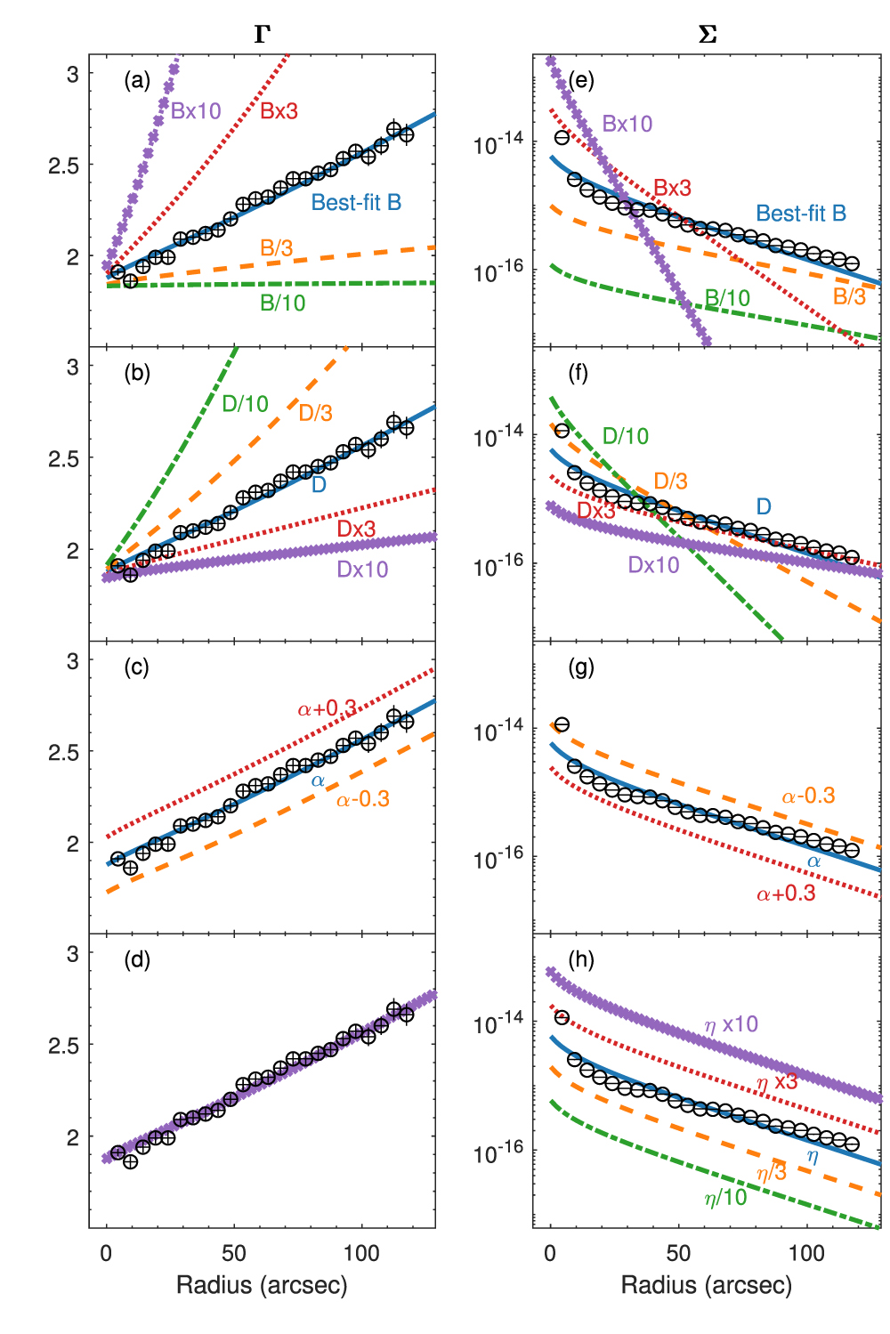
Based on our pure diffusion model with transmitting boundary, three parameters are critical for the Γ profile: B-field in the PWN, D, and the injected power-law index α of the particle energy. Moreover, η plays an important role in the Σ profile. However, the B-field strength is a predefined value and varies dramatically among studies; see, e.g., G21 (Tanaka & Takahara 2011, 2013; Guest et al. 2019). This parameter is coupled with D, and therefore it is meaningless to directly compare D among PWNe. Taking 3C 58 as an example, we demonstrate how the model profile changes as we change these parameters in Figure 3. From Figures 3(a) and (b), the effects of B and D are coupled with each other (Tang & Chevalier 2012). A flatter Γ profile, which implies a lower energy dissipation, can be achieved by both decreasing B and increasing D, and vice versa. This is because the spatial extent of the X-ray-emitting particles is defined by the distance over which they spread before exhausting their energy via synchrotron radiation. The ratio of the diffusion length of a particle emitting a photon of a given frequency ν to a radius R can be written as , where tcool = 1/QE is the cooling timescale of the synchrotron emission. The Σ profile is the same if DB−3/2 remains constant. Therefore, DB−3/2 is the key parameter for the shape of the Γ profile. Since the PWN B-field strength is difficult to estimate and it often depends on many assumptions, we will not discuss the effect of D. Instead, we focus on DB−3/2 in the following discussions. The DB−3/2 values of the sampled PWNe are listed in Table 2. The Γ fitting results of 3C 58 and G21.5−0.9 are in the same order as those derived in Tang & Chevalier (2012) with full synchrotron spectrum.


Figure 3. Parameter dependence of model profiles in (a–d) Γ and (e–h) Σ in units of erg cm−2 s−1 arcsec−2. Data points are results from 3C 58.
Download figure:
Standard image High-resolution imageWe further test the sensitivity of the effect of parameters on the Σ profile (Figures 3(e) and (f)). The DB−3/2 value changes not only the shape but also the displacement (or interception) of model profiles. Comparing to the Γ profile, we notice that the shape of the Σ profile becomes insensitive to DB−3/2 as long as DB−3/2 is large enough. From Figure 3(c), the offset of Γ, which implies the general hardness of the PWN, is dominated by α of the injected high-energy particles. On the other hand, the displacement of the Σ profile could be affected by DB−3/2, α, and η. Finally, η only affects the displacement in the Σ profile because it represents the energy-transferring efficiency from the spin-down power of the pulsar to the PWN.
6.3. Profile Characteristics and Model Parameters
Based on the discussion in Section 6.2, we test whether the characteristics, i.e., slope and mean value of the Γ and Σ profiles, can be interpreted with the pure diffusion parameters. To achieve this goal, we simply fit the Γ profile of each PWN with a straight line. Crab and Vela are not included in this analysis since their profiles cannot be described with our model. The slope can roughly represent the Γ gradient. We take the mean of Γ as the value at the half of the PWN radius predicted from the best-fit straight line. For the Σ profile, we define the same slope and the mean Σ as we did for the Γ profile. The difference is that we use the logarithmic scale for the surface brightness.
Then, we plot the apparent features (slope and mean value of the Γ and the Σ profiles) versus the model parameters in Figure 4. The most significant correlation is, not surprisingly, between the mean of Γ and α. The linear correlation coefficient is ρ = 0.89 with a null hypothesis probability p = 0.006 for the Γ fit, where the Σ fitting result is ρ = 0.96 with p = 6 × 10⁻⁴. A relatively weak correlation can be seen between DB−3/2 and the slope of the Γ profiles with ρ = −0.85 and p = 0.02 for the Γ fit. The correlation is insignificant for the Σ fit with ρ = −0.40 and p = 0.3. This is caused by the large discrepancy between the Γ and Σ fitting results of a few PWNe where the Σ fit cannot well describe the Γ profile.

Figure 4. Correlation between model parameters and apparent parameters of the Γ and Σ profiles. Gray circles denote the parameters derived from the Γ fit, while the red triangles are parameters from the Σ fit. We use a blue line to link the parameters obtained by Γ and Σ fits for each PWN.
Download figure:
Standard image High-resolution imageThe slope of the Σ profile is correlated with DB−3/2, where the correlation analysis suggests ρ = 0.75 and p = 0.05 for both the Σ and Γ fits. The relation between these two parameters might be nonlinear. Therefore, we also calculate Kendall's rank correlation and obtain a Kendall's τ = 0.81 with p = 0.01 for the Γ fit and τ = 0.52 with p = 0.1 for the Σ fit. This suggests a possible correlation and is consistent with the result in Section 6.2, in which we show that a larger D (or smaller B) results in a flatter Σ profile. Interestingly, the slope of the Σ profile anticorrelates with η with ρ = −0.84 and p = 0.01 for the Σ fit (ρ = −0.88 and p = 0.009 for the Γ fit), suggesting a similar significance to that between DB−3/2 and the Σ profile. This is not expected, as we discussed in Section 6.2, and could indicate a physical connection underneath. Finally, the mean surface brightness likely anticorrelates with DB−3/2 and positively correlates with η; these are expected in Section 6.2. However, the mean surface brightness does not correlate with α, suggesting that α is not the dominant factor for the Σ profile.
6.4. Correlation between Model Parameters and Physical Parameters
We tested whether the best-fit parameters and physical parameters correlate with each other. We performed correlation analysis between four parameters, including DB−3/2, α, η, and the PWN age. The results are shown in Figure 5. It is worth mentioning that η of Kes 75 is the largest among the selected PWNe. Given that PSR J1846−0258 is a high B-field pulsar that shows a magnetar-like burst and outburst behavior, it is possible that the dissipation of the extremely strong magnetic field results in additional energy output from the pulsar (Gavriil et al. 2008; Kumar & Safi-Harb 2008; Ng et al. 2008).

Figure 5. Correlation between model parameters and physical parameters. Gray circles denote the parameters derived from the Γ fit, while red triangles are parameters from the Σ fit. We use a blue line to link the parameters obtained by Γ and Σ fits of each PWN. The ages of PWNe and Lsd are adopted from Table 1.
Download figure:
Standard image High-resolution imageIn general, we found no significant correlations between these parameters, indicating that these parameters are independent of each other. We found that DB−3/2 may weakly anticorrelate with with ρ = −0.7 and p = 0.07 for the Γ fit. This possible correlation is not observed for the Σ fit with ρ = −0.5 and p = 0.3, suggesting no significance. We could not draw a strong conclusion with our current sample. However, this could be connected to the anticorrelation between the slope of the brightness profile and η in Section 6.3. A larger DB−3/2 implies a steeper Γ gradient in the radial profile, i.e., stronger synchrotron energy loss. Therefore, a high energy conversion rate might not be needed.

7. Summary
We applied a pure diffusion model to fit the Γ and Σ profiles of nine young PWNe, including well-studied 3C 58 and G21.5−0.9; a few faint sources, G54.1+0.3, G291.0−0.1, G310.6−1.6, and Kes 75; and three bright PWNe, Crab, MSH 15−52, and Vela. We analyzed archival Chandra observations and fit the spectra of each PWN with a power-law model. Except for Crab and Vela, all the sampled PWNe show similar Γ and Σ profiles. Γ increases slowly with the distance from the central pulsar. This behavior cannot be described by the MHD model, which suggests an abrupt increase in Γ (Slane et al. 2004; Tang & Chevalier 2012; Ishizaki et al. 2017) and therefore suggests that particle diffusion dominates the particle transfer rather than a steady flow for most PWNe. We derived the brightness profile from the pure diffusion model and found that the observed profiles are consistent with the model prediction. However, the parameters that can describe the Γ profile and those for the Σ profiles are not consistent with each other in a few cases like 3C 58 and G54.1+0.3. The discrepancy implies that a simple diffusion model may not be enough to produce the entire distribution of PWNe and future improvement is necessary. The discrepancy could be attributed to the intrinsic spherical asymmetry, the particle reflection by the PWN boundaries, energy-dependent diffusion, and spatially dependent B-field. The last two could be specified with multiwavelength studies. A model with a spatially varying magnetic field could be constructed in the future. We further investigate the relationship between the model parameters and the apparent feature of both profiles. The effects of the diffusion coefficient and the magnetic field are coupled with each other, and the observed Γ and the Σ gradient highly depend on the DB−3/2 value. The mean hardness of a PWN significantly correlates with the distribution of the injected particles, while the brightness of a PWN is dominated by the energy conversion efficiency η. Finally, we found no significant correlations between model parameters and the physical quantities of PWNe.
We thank the anonymous reviewer for valuable comments that improved this paper. This research is based on the data obtained from the Chandra Data Archive and has made use of the software provided by the Chandra X-ray Center (CXC) in the application packages CIAO, ChIPS, and Sherpa. C.-P.H. acknowledges support from the Ministry of Science and Technology in Taiwan through grant MOST 109-2112-M-018-009-MY3. W.I. is supported by JSPS KAKENHI grant No. 21J01450. C.-Y.N. is supported by a GRF grant of the Hong Kong Government under HKU 17305416. S.J.T. acknowledges support by the Aoyama Gakuin University-Supported Program "Early Eagle Program."
Facility: CXO (ACIS). -
Software: CIAO (Fruscione et al. 2006), Sherpa (Freeman et al. 2001).
Appendix A: Data Sets Used in This Research
We list all data sets used in this analysis in Table A1.
Table A1. Chandra Observation Log of Selected PWNe
| PWN Name | ObsID | Date | Exposure (ks) |
|---|---|---|---|
| 3C 58 | 728 | 2000-09-14 | 38.7 |
| 4383 | 2003-04-22 | 38.7 | |
| 4382 | 2003-04-23 | 167.4 | |
| 3832 | 2003-04-26 | 135.8 | |
| G21.5−0.9 | 159 | 1999-08-23 | 14.9 |
| 1230 | 1999-08-23 | 14.6 | |
| 1433 | 1999-11-15 | 15.0 | |
| 1716 | 2000-05-23 | 7.7 | |
| 1717 | 2000-05-23 | 7.5 | |
| 1718 | 2000-05-23 | 7.6 | |
| 1769 | 2000-07-05 | 7.4 | |
| 1770 | 2000-07-05 | 7.2 | |
| 1771 | 2000-07-05 | 7.2 | |
| 1838 | 2000-09-02 | 7.9 | |
| 1839 | 2000-09-02 | 7.7 | |
| 1553 | 2001-03-18 | 9.8 | |
| 1554 | 2001-07-21 | 9.1 | |
| 2873 | 2002-09-14 | 9.8 | |
| 3693 | 2003-05-16 | 9.8 | |
| 3700 | 2003-11-09 | 9.5 | |
| 5166 | 2004-03-17 | 10.0 | |
| 5159 | 2004-10-27 | 9.8 | |
| 6071 | 2005-02-26 | 9.6 | |
| 6741 | 2006-02-22 | 9.8 | |
| 8372 | 2007-05-25 | 10.0 | |
| 10646 | 2009-05-29 | 9.5 | |
| 14263 | 2012-08-08 | 9.6 | |
| 16420 | 2014-05-07 | 9.6 | |
| G54.1+0.3 | 1983 | 2001-06-06 | 38.5 |
| 9886 | 2008-07-08 | 65.3 | |
| 9108 | 2008-07-10 | 34.7 | |
| 9109 | 2008-07-12 | 162.3 | |
| 9887 | 2008-07-15 | 24.8 | |
| G291.0−0.1 | 2782 | 2002-04-08 | 49.5 |
| 16497 | 2013-10-28 | 37.6 | |
| 14822 | 2013-11-03 | 51.5 | |
| 14824 | 2013-11-04 | 74.1 | |
| 14823 | 2013-11-10 | 67.0 | |
| 16512 | 2013-11-13 | 63.4 | |
| 16541 | 2014-01-21 | 29.2 | |
| 16566 | 2014-02-15 | 34.6 | |
| G310.6−1.6 | 9058 | 2008-06-29 | 5.1 |
| 12567 | 2010-11-17 | 52.8 | |
| 17905 | 2016-11-25 | 13.9 | |
| 19919 | 2016-11-29 | 79.7 | |
| 19920 | 2016-12-05 | 39.46 | |
| Kes 75 | 748 | 2000-10-15 | 37.3 |
| 7337 | 2006-06-05 | 17.4 | |
| 6686 | 2006-06-07 | 54.1 | |
| 7338 | 2006-06-09 | 39.3 | |
| 7339 | 2006-06-12 | 44.1 | |
| 10938 | 2009-08-10 | 44.6 | |
| 18030 | 2016-06-08 | 85.0 | |
| 18866 | 2016-06-11 | 61.5 | |
| MSH 15−52 | 754 | 2000-08-14 | 19.0 |
| 3834 | 2003-04-21 | 9.5 | |
| 4384 | 2003-04-28 | 9.9 | |
| 3833 | 2003-10-17 | 19.1 | |
| 5334 | 2004-12-28 | 49.5 | |
| 5335 | 2005-02-07 | 42.6 | |
| 6116 | 2005-04-29 | 47.0 | |
| 6117 | 2005-10-18 | 45.6 | |
| Vela | 128 | 2000-04-30 | 10.6 |
| 1987 | 2000-11-30 | 18.9 | |
| 2813 | 2001-11-25 | 17.9 | |
| 2814 | 2001-11-27 | 19.9 | |
| 2814 | 2001-12-04 | 27.0 | |
| 2816 | 2001-12-11 | 19.0 | |
| 2817 | 2001-12-29 | 18.9 | |
| 2818 | 2002-01-28 | 18.7 | |
| 2819 | 2002-04-03 | 19.9 | |
| 2820 | 2002-08-06 | 19.5 | |
| 3861 | 2003-08-21 | 4.9 | |
| 10132 | 2009-07-09 | 39.5 | |
| 10133 | 2009-07-17 | 39.5 | |
| 10134 | 2009-07-25 | 38.1 | |
| 10135 | 2010-06-28 | 39.5 | |
| 10136 | 2010-07-08 | 39.5 | |
| 10137 | 2010-07-17 | 39.5 | |
| 10138 | 2010-07-26 | 38.8 | |
| 10139 | 2010-08-04 | 39.5 | |
| 12073 | 2010-08-15 | 39.5 | |
| 12074 | 2010-08-24 | 39.5 | |
| 12075 | 2010-09-04 | 41.8 | |
| Crab | 14458 | 2012-11-26 | 1.24 |
| 14679 | 2013-01-02 | 0.66 | |
| 14680 | 2013-02-25 | 0.66 | |
| 14685 | 2013-03-07 | 0.61 | |
| 14681 | 2013-04-23 | 0.61 | |
| 14682 | 2013-08-16 | 0.61 | |
| 14678 | 2013-10-08 | 0.63 | |
| 16245 | 2013-10-19 | 1.29 | |
| 16257 | 2013-11-04 | 1.29 | |
| 16357 | 2014-01-29 | 1.3 | |
| 16358 | 2014-04-19 | 1.32 | |
| 16359 | 2014-08-16 | 1.32 | |
| 16258 | 2014-11-06 | 1.34 | |
| 16360 | 2015-01-18 | 1.37 | |
| 16361 | 2015-04-10 | 1.42 | |
| 16362 | 2015-08-60 | 1.44 | |
| 16259 | 2015-11-06 | 1.44 | |
| 16363 | 2016-01-31 | 1.44 | |
| 16364 | 2016-04-20 | 1.43 | |
| 16365 | 2016-08-14 | 1.51 | |
Appendix B: CHANDRA Images and Spectral Extraction Regions
Figure A1 shows the Chandra 0.5–8 keV images of all the sampled PWNe. To study the radial profile, we use multiple annuli centered on the central pulsar to select X-ray photons and collect X-ray spectra.

Figure A1. Chandra 0.5–8 keV image of (a) 3C 58, (b) G21.5−0.9, (c) G54.1+0.3, (d) G291.0−0.1, (e) G310.6−1.6, (f) Kes 75, (g) MSH 15−52, (h) Vela, and (i) Crab. The green annuli denote the selected areas for spectral analysis. The jets, clumps, and background stars are removed.
Download figure:
Standard image High-resolution image