


Abstract
The presence of the ≈106 K gas in the circumgalactic medium of the Milky Way (MW) has been well established. However, the location and the origin of the newly discovered hot gas at "supervirial (SV)" temperatures of ≈107 K have been puzzling. This hot gas has been detected in both absorption and emission; here, we focus on the emitting gas only. We show that both the "virial" and the SV temperature gas, as observed in emission, occupy disk-like extraplanar regions, in addition to the diffuse virial temperature gas filling the halo of the MW. We perform idealized hydrodynamical simulations to show that the ≈107 K emitting gas is likely to be produced by stellar feedback in and around the Galactic disk. We further show that the emitting gas at both SV and virial temperatures in the extraplanar regions is metal enriched and is not in hydrostatic equilibrium with the halo but is continuously evolving.

Original content from this work may be used under the terms of the Creative Commons Attribution 4.0 licence. Any further distribution of this work must maintain attribution to the author(s) and the title of the work, journal citation and DOI.
1. Introduction
The gas surrounding the stellar disk and the interstellar medium (ISM) of a galaxy is referred to as the "circumgalactic medium" (CGM; for a review, see J. Tumlinson et al. 2017; S. Mathur 2022; C.-A. Faucher-Giguère 2023). Observations of the CGM of the Milky Way (MW) and other galaxies, as well as numerical simulations, suggest the presence of multiphase gas in the CGM, with a large range in density and temperature. The gas temperature varies from the cold phase (∼104 K) to the virial phase (∼106 K). The "virial gas" (∼106 K or 0.2 keV), so called because its temperature is comparable to the MW virial temperature, is the volume-filling and the most massive component of the CGM, and is detected in X-rays in both absorption and emission (A. Gupta et al. 2012). Gas in the cold (104 K) and warm (105 K) phases is detected in the optical/UV band in absorption using bright background sources (typically a quasar).
Recent observations have, however, indicated the presence of ∼107 K (0.8 keV) gas in addition to the gas at lower temperatures. Following S. Das et al. (2021), we refer to this ∼107 K gas as the "supervirial" (SV)" gas (instead of "coronal" or "hot" gas, to avoid confusion with the ∼106 K gas). We will make further distinctions regarding this phase as follows. We will refer to the SV phase that has been detected using Si xiv and Ne x absorption lines in the X-ray spectra of background quasars along a few lines of sight (S. Das et al. 2019b, 2021; A. Lara-DI et al. 2023; R. L. McClain et al. 2024; A. Lara-DI et al. 2024), as "SV absorption." And by "SV emission" we will refer to the hot gas that has been detected in the emission studies of the MW CGM in many fields across the sky, in addition to the virial phase. In this paper, we will focus on the SV emission phase, and the case of SV absorption will be dealt with in a separate paper.
Several X-ray observatories (e.g., Chandra (M. C. Weisskopf et al. 2000), XMM-Newton (F. Jansen et al. 2001), Suzaku (K. Mitsuda et al. 2007), HaloSat (P. Kaaret et al. 2019), eROSITA (P. Predehl et al. 2021)) have been put into service for these emission observations. S. Das et al. (2019a) detected the SV phase in the MW CGM using XMM-Newton observation toward the blazar IES 1553+113 (l = 21 91, b = 4396) in emission. They fitted the total emission from the CGM with a two-temperature thermal plasma model. Assuming solar metallicity, their best-fitted values of two temperatures are 0.15−0.23 and 0.41−0.72 keV. A. Gupta et al. (2021) used Suzaku and Chandra observations of the MW halo to characterize the emission along four sightlines. Again, for solar metallicity, they found the two temperatures to be 0.176 ± 0.008 keV and 0.65–0.90 keV. J. Bhattacharyya et al. (2023) used XMM-Newton observation toward the Blazar Mrk 421 (l = 17983, b = 6503) and five other sightlines near the blazar field to study the emission from MW CGM. Using solar metallicity to analyze their observation, they found the temperature of the two phases to be 0.14–0.192 keV and 0.66–1.14 keV. J. Bluem et al. (2022) used the HaloSat all-sky survey to study the emission from the MW halo. Assuming 0.3 solar metallicity, they obtained the average temperature of and 0.184 ± 0.009 keV for northern and southern virial gas, respectively. For the SV gas, the average temperature is and 0.75 ± 0.08 keV, respectively. G. Ponti et al. (2023) observed the MW halo in the eFEDDS field using eROSITA. Their best-fit metallicity was 0.068 Z⊙ for the virial phase, much less than the value of 0.3 Z⊙ that is often used in CGM studies. However, they used 0.7 solar metallicity for the SV gas. H. Sugiyama et al. (2023) studied emission from the MW halo with Suzaku using 130 observations. They used solar metallicity in the SV phase for their analysis. Lastly, A. Gupta et al. 2023 analyzed the X-ray emitting gas in the CGM using 230 Suzaku archival observations. Assuming solar metallicity, they found the temperature of virial and super-virial gas to be ∼0.2 and ∼0.4–1.1 keV respectively. All these observations show that the SV hot phase of MW CGM, as observed in emission, is ubiquitous across the sky. While a two-temperature model provided the best fit to all these data, there is clearly some scatter in the temperature of both the virial and SV phases, suggesting a multiphase nature of CGM.


Recently, C. A. Fuller et al. (2023) observed and analyzed the emission from the Orion–Eridanus Superbubble and found the temperature and emission measures (EMs) of the gas in this region to be similar to the bulk gas in the CGM elsewhere. This result suggests that the SV gas is likely associated with core-collapse supernovae (SNe)-driven outflow from the Galactic disk. In this paper, we model the SV gas (∼107 K) and the virial gas (∼106 K) with disk-like profiles, in addition to the extended CGM at the virial temperature. The unique feature of our model is the extraplanar disk-shaped region containing both SV and virial gas. These two gas phases need not be in hydrostatic equilibrium and are likely to be in a dynamical state. We explain the physical nature of the coexistence of these two phases around the disk, using an idealized numerical simulation of star formation-driven outflows in a MW-type galaxy. Our paper is organized as follows. Section 2 introduces our model, followed by a description of the simulation setup and results in Sections 3 and 4. We discuss the implications in Section 5 and finally summarize our work in Section 6.
2. Disk-shaped Profile of the Virial and SV Gas
To begin with, we seek clues for the possible geometric shape of the region occupied by the SV emission phase. P. Kaaret et al. (2020), N. Locatelli et al. (2024), A. Dutta et al. (2024), and S. Nakashima et al. (2018) have argued that the CGM emission is best described by a disky extraplanar component. In Figure 1 we have plotted the observed EMs of the virial and the SV temperature gas as a function of sin (b), where b is the Galactic latitude for various observations. The black solid lines show the mean EM for both the virial and SV phases calculated in a bin size of . We see an anticorrelation of EM with sin (b), as expected for a disk-shaped region, for both the virial and SV phases, as depicted by the trend in black solid lines. We have performed Kendall's tau test to quantify the anticorrelation. For the virial phase, we obtain τ = −0.20 and a p-value = 10−4, where τ is the correlation coefficient and the p-value signifies the probability of the null hypothesis. The τ/p-value = 1/0 signifies a strong correlation, while τ/p-value = 0/1 signifies no correlation. For the SV phase, we obtain τ = −0.18 and p-value = 5 × 10⁻⁴. The finite negative τ values signify the anticorrelation.

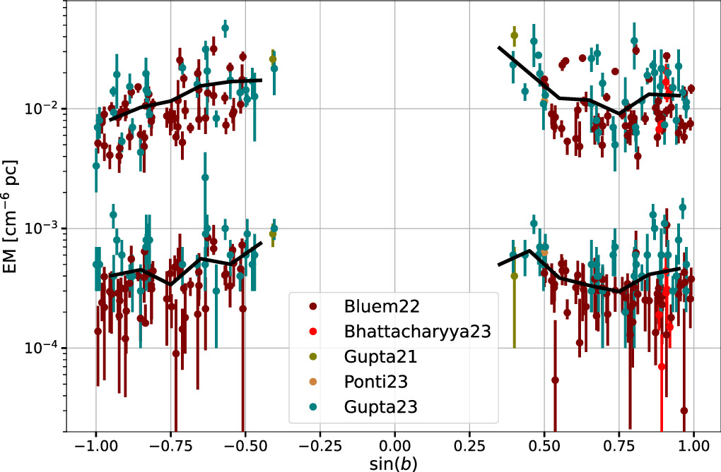
Figure 1. The EM data from various authors (A. Gupta et al. 2021; J. Bluem et al. 2022; G. Ponti et al. 2023; J. Bhattacharyya et al. 2023 and A. Gupta et al. 2023) is plotted as a function of sin (b), where b is the Galactic latitude. The figure contains two sets of data. The top set of points, with EM ≈ 10−3−10−1 cm−6 pc, corresponds to the virial phase, while lower data points with EM ≈ 10−5−10−3 cm−6 pc correspond to the SV phase. The solid black lines show the mean EM calculated in a bin size of for both the virial and SV data sets. Note the anticorrelation between EM and sin (b) for both the virial and SV phases, as can be seen by the trend in the black solid lines.

Download figure:
Standard image High-resolution imageJ. Bluem et al. (2022) and J. Bhattacharyya et al. (2023) have shown that the EMs of the SV and virial phases are correlated, suggesting that they are cospatial. Thus, it appears that both viral and SV-phase emission may arise in an extraplanar disk around the Galactic disk. A disk-like profile of the SV phase is also a natural outcome of the stellar activities in the disk of the MW, as we show in Section 4. However, in order to understand the virial phase absorption, an extended diffuse component is required (A. Gupta et al. 2012, 2014).
With this in mind, we set up our geometric model, as shown in Figure 2. It shows a schematic representation of our model of the extraplanar gas around the MW. The blue slab shows the Galactic ISM. The regions with magenta and yellow colors show the extent of the SV and virial disks, respectively. The extended spherical green region shows the virial temperature CGM in the Galactic halo. Note that the regions in the figure are not to scale and are only schematic in nature. In what follows, we determine the parameters of these three geometric shapes.

Figure 2. The cartoon representation of the structure of the gaseous components of the MW. The blue region in the center shows the ISM. The magenta and the yellow regions show the extent of the SV and virial temperature-emitting disks, respectively. The extended region in green shows the Galactic-virialized halo. Note that the size of different regions is not to scale; it simply represents the overall structure of the extraplanar gas around the MW.
Download figure:
Standard image High-resolution imageFirst, let us consider the volume-filling diffuse gas in the Galactic halo at the virial temperature. Consider the halo gas in hydrostatic equilibrium with the dark matter potential of the MW, for which we use the Navarro–Frenk–White (NFW) profile (J. F. Navarro et al. 1997). We further assume the halo gas to be at a uniform temperature of 3 × 10⁶ K (isothermal sphere) for simplicity. Although other halo profiles are also possible (A. H. Maller & J. S. Bullock 2004; M. J. Miller & J. N. Bregman 2013; G. M. Voit 2019; Y. Faerman et al. 2020), we use the simplest model to minimize the number of free parameters.
We obtain the following equation for the halo gas density profile:

where x = r/rs (rs is the scale radius in the NFW profile), n0 is the density at the center, and (C being the concentration parameter). We use Mvir = 1012 M⊙, C = 12, rvir = 260 kpc (A. Klypin et al. 2002), and T = 3 × 10⁶ K, for which f0 = 3. The central density n0 is obtained from the normalization condition that the total baryonic mass in the CGM (1.2 × 10¹¹ M⊙) is 75% of the total baryonic mass in MW (J. X. Prochaska & Y. Zheng 2019), assuming cosmic baryonic fraction of 0.16. This gives n0 = 8.8 × 10⁻⁴ cm−3.
![${f}_{0}=G\mu {m}_{p}{M}_{\mathrm{vir}}/[{k}_{B}{{Tr}}_{s}\{\mathrm{ln}(1+C)-C/(1+C)\}]$](https://content.cld.iop.org/journals/0004-637X/975/1/49/revision1/apjad77c0ieqn5.gif)
With this, we calculate the EM (EM = ∫ne nH d l) of the virial temperature halo gas. We used μ = 0.67, μe = 1.18, and μH = 1.22 such that n μ = ne μe = nH μH. We then subtract the halo EM from the total EM of the virial temperature gas so as to determine the EM from the disk component. We note that the halo contributes only 30% on average to the total EM of the virial phase.
The disk-like model for the extraplanar profile of the virial temperature gas is given by

where nV is the total number density at the Galactic center for the virial phase, zV is the scale height, and RV is the scale radius. Note that the density profile is exponential in the z-direction only below RV , while above RV , it is exponential in both the R- and z-directions, where R and z are the cylindrical coordinates.
Similarly, we model the extraplanar SV gas profile with a disk-like shape as follows:

where nSV is the total number density at the Galactic center for the SV phase, zSV is the scale height, and RSV is the scale radius.
To determine the parameters of the disk profiles of both phases, we perform Markov Chain Monte Carlo (MCMC) analysis using emcee (D. Foreman-Mackey et al. 2013) for the observed EMs reported in the literature (S. Das et al. 2019a; A. Gupta et al. 2021; J. Bluem et al. 2022; A. Gupta et al. 2023; G. Ponti et al. 2023 and J. Bhattacharyya et al. 2023). To obtain the parameters for the extraplanar virial gas, we subtract the EM contribution from the extended halo virial gas profile (see Equation (1), isothermal profile) and use the residual EM values as the observed data, as discussed earlier in the section. We assume 0.3 solar metallicity for the virial phase (S. Toft et al. 2002; J. Sommer-Larsen 2006; J. X. Prochaska et al. 2017) and solar metallicity for the SV phase (motivated by the fact that the SV phase is likely the result of outflows from core-collapse SNe in the MW disk). We accordingly scale the observed EM values as . We performed MCMC analysis separately for the extraplanar virial and SV gas. We use Gaussian priors for all the parameters with 32 walkers and 50,000 steps. We ensured the convergence of the samples as the number of steps (50,000 in this case) is larger than 50 times the autocorrelation time. In Table 1, we show the allowed range, initial guess value, line center, and width of the Gaussian priors, and the results of all the parameters in MCMC analysis for both the virial and SV phases. Figure 3 shows the corner plot of MCMC analysis. We find that the parameters of the extraplanar profiles for both the SV and virial phases are similar, with comparable values for the scale heights and scale radii, although the densities are different. The virial phase emission is significantly brighter (higher EM) compared to the SV phase, resulting in a higher density for the virial phase.


Figure 3. This figure shows the results of the MCMC analysis. The left and right panel shows the corner plot of parameters for virial and SV phases respectively. The three vertical dashed black lines in the 1D histogram mark the 16th, 50th, and 84th percentiles of the samples. The three contour levels plotted with black solid lines contain 32%, 64%, and 96% of the samples, respectively. The blue line shows the initial guess value and is visible only in the case of zv, as the guess values for other parameters are out of the plot ranges. The values on the top of each 1D histogram show the 50th percentile value (median) and the error shown corresponds to 16th and 84th percentiles, which is equal to a 1σ error if the resulting 1D histogram is Gaussian, which is the case for most of the parameters. We performed the analysis using 32 walkers and 50,000 steps with Gaussian priors for all the parameters. We ensured the convergence of samples as the total number of steps are larger than 50 times the autocorrelation time. Note that the width in the Gaussian prior (see Table 1) is sufficiently larger than the width in the resulting histogram of the respective parameters. This shows that the resulting values are well constrained.
Download figure:
Standard image High-resolution imageTable 1. Allowed Range, Initial Guess Values, Line Center, and Width in the Gaussian Priors of the Parameters for the MCMC Analysis
| Parameter | Allowed Range | Initial Guess | Gaussian Line Center | Gaussian Half-width | Results | |||
|---|---|---|---|---|---|---|---|---|
| V/SV | V | SV | V | SV | V/SV | V | SV | |
| (cm−3)] | [−5, −0.1] | −2 | −3 | −1.5 | −2.5 | 5 | ||
| R (kpc) | [1, 15] | 4.5 | 6 | 5 | 4 | 10 | ||
| z (kpc) | [0.1, 10] | 1.5 | 2.0 | 1.0 | 1.5 | 10 | ||


Note. The last column shows the result of the MCMC analysis for the virial (V) and the SV phases. The values shown are the median values (50th percentile) with uncertainties equal to 16th and 84th percentiles (1σ).
Download table as: ASCIITypeset image
Using the results of the MCMC analysis for the disk-shaped virial and SV gas and the extended volume-filling halo virial gas using Equation (1), we calculated the EMs for both the virial and SV phases along the observed lines of sight. Figure 4 shows the EM correlation of the two phases. The black open circles show the correlation with the halo virial profile along with extraplanar SV gas. The blue circles correspond to the extraplanar virial and SV gas (and no halo gas). The circles in cyan show the correlation in the presence of a halo virial, extraplanar virial, and extraplanar SV gas. The observed EM from various authors are plotted with different colors: J. Bluem et al. (2022) in maroon, A. Gupta et al. (2023) in green, J. Bhattacharyya et al. (2023) in red, A. Gupta et al. (2021) in olive, G. Ponti et al. (2023) in peru, and S. Das et al. (2019a) in magenta.

Figure 4. The correlation between the EM of the virial temperature gas and the EM of the SV temperature gas based on our models overplotted on observed EM. The black open circles show the EM correlation for the virial halo profile and SV gas in the extraplanar region. The blue circles show the EM correlation with the extraplanar virial and SV gas. The circles in cyan correspond to the virial gas in the halo + the virial gas and the SV gas in the extraplanar regions around the Galactic disk. The EM values from our model are plotted for the observed lines of sight. The observational data points from various authors are shown in other colors with error bars. All the observed EM values are rescaled to the metallicity of 0.3 solar for virial gas and solar for SV gas. The narrow range in the black points compared to cyan points along the X-axis shows the importance of having a "disk-shaped" virial phase profile.
Download figure:
Standard image High-resolution imageIt is clear from Figure 4 that the model without extraplanar virial gas (black open circles) cannot explain the observed data; a disk-like extraplanar region with virial temperature gas is required. The observed correlation is well explained by the extraplanar SV and virial gas model with an extended virial halo profile (cyan-colored circles). The total mass in the disk-like extraplanar region (Equations (2), (3)) is , where n0 is the central density in cm−3, z0 and R0 are the scale height and scale radius in kpc respectively. We calculated the mass in the extraplanar virial and the SV phase using the best-fit parameters from Table 1. We obtain 1.7 × 10⁸ M⊙ and 3.5 × 10⁷ M⊙ for the two phases, respectively. Note that this is insignificant compared to the mass of the virial gas in the halo, and therefore, does not affect the hydrostatic equilibrium that was assumed to obtain Equation (1). The baryonic mass of the CGM is dominated by the extended, diffuse gas filling the Galactic halo.

3. Simulation Setup
In Section 2, we determined the location of the virial and SV phases in emission, measured the parameters of the extraplanar disks, measured the density profiles, calculated the EMs, and determined masses in these phases. This answers the question: "Where is the hot gas?" However, this does not tell us why. A likely answer is the feedback from the stellar disk. In order to understand the origin of the SV-phase gas, we have built a model of the outflows from the OB associations in the MW disk. We perform a hydrodynamical simulation of outflows from the MW disk and show that the extraplanar SV gas may indeed arise from the feedback.
We performed our simulation in 2D cylindrical coordinates (R and z), using the publicly available hydrodynamical code PLUTO (A. Mignone et al. 2007). Our initial Galactic setup is similar to that of K. C. Sarkar et al. (2015) with a rotating ISM and nonrotating isothermal CGM in the gravitational field of an NFW halo (J. F. Navarro et al. 1997) and Miyamoto–Nagai disk (M. Miyamoto & R. Nagai 1975). The temperature, density, and pressure initial conditions are as shown in Figure 5. The cold ISM is at T = 4 × 10⁴ K and the CGM is at T = 3 × 10⁶ K. The temperature gradient, as shown in Figure 5 allows for a stable thermal configuration, for the gravitational forces to be supported by gas pressure and rotation, as discussed in K. C. Sarkar et al. (2015). We use the Harten–Lax–van Leer Riemann solver and resolve the time using the Runge–Kutta second-order scheme.

Figure 5. The initial temperature, density, and pressure maps. There are temperature and density gradients in both the R- and z-directions, as a result of the hydrostatic equilibrium in which the gravitational force is balanced by gas pressure combined with the rotation of the gas.
Download figure:
Standard image High-resolution imageGrid: We define our simulation box from 10 pc to 30 kpc along the R-direction. We take a uniform grid from 10 pc to 10 kpc (450 grid points) and a logarithmic grid from 10 kpc to 30 kpc (62 grid points). In the z-direction, we define our computational box from 1 pc to 30 kpc with a uniform grid from 1 pc to 10 pc (20 grid points) and then logarithmic grids from 10 pc to 30 kpc (236 grid points).
Boundary condition: We use reflective boundary conditions for inner boundaries in both the R- and z-directions. For the outer boundary in both R and z, pressure and density values are set to initial equilibrium values, whereas velocity values are copied from the nearest active zones. We set an "axisymmetric" boundary condition in the ϕ-direction.
Cooling: We do not allow the Galactic ISM (R < 15 kpc and z < 2 kpc) to cool. However, we allow the injected and CGM gas to cool, using a radiative cooling function. The metallicity for the injected material and CGM gas is set at 1 Z⊙ and 0.3 Z⊙, respectively. We set the cooling to be tabulated and use the radiative transfer code CLOUDY (G. J. Ferland & M. Chatzikos et al. 2017) to obtain the cooling rates.
Various studies have shown that star-forming regions of the MW are not concentrated in the Galactic center but are distributed in rings in the Galactic plane with a peak of star formation around 4–5 kpc (e.g., D. Elia et al. 2022). Motivated by these observations, we injected mass and energy into the Galactic disk rather than solely in the Galactic center. The star formation rate (SFR) density has been measured in concentric rings of widths 0.5 kpc by D. Elia et al. (2022; see their Figure 6). For our calculation, we use these measurements in rings up to 10 kpc. We computed the SFR in each bin using the observed SFR density and the relevant area of the ring. The estimated SFR in the rings, starting from the center, is 0.035, 0.018, 0.011, 0.016, 0.015, 0.038, 0.048, 0.093, 0.174, 0.201, 0.170, 0.158, 0.184, 0.125, 0.079, 0.074, 0.076, 0.068, 0.045, and 0.055 M⊙ yr−1, respectively.

Figure 6. Temperature maps at three epochs, at 5, 10, and 15 Myr, from left to right. As the energy is injected into the disk, the hot SV temperature gas is pushed up, generating an extraplanar region (shown in blue). Above this region, a virial temperature extraplanar region is formed (shown in yellow-green). Shock heating of the halo gas leads to another hot region at higher z (shown in light green).
Download figure:
Standard image High-resolution imageEnergy and mass injection: We inject mass and energy in 20 cylindrical rings (of height 10 pc and width 0.5 kpc) up to 10 kpc centered around 0.25, 0.75, ...9.25, and 9.75 kpc. The amount of mass and energy injected in each bin depends on the SFR of the bin (as mentioned above). Note that this is similar to A. Vijayan et al. (2018) except that we use the observed SFR in each bin from D. Elia et al. (2022), whereas A. Vijayan et al. (2018) used gas density to infer the SFR using the Kennicutt–Schmidt relation (R. C. J Kennicutt 1998). Assuming that each supernova (SN) releases 1051 erg of energy, the relation between mechanical luminosity and SFR is

where is the number of SNe per unit mass of the stars formed, and  is the heating efficiency of the gas. Assuming a Salpeter initial mass function (E. E. Salpeter 1955) between the lower and upper limit on a stellar mass of 0.1 and 100 M⊙, respectively, we get . Thus, the relation becomes


We assume = 0.3, which takes into account the radiative loss of energy (E. O. Vasiliev et al. 2015; N. Yadav et al. 2017). This quantifies the amount of energy being injected in each bin. We inject total energy in the thermal form.
The corresponding mass injection rate is quantified by the "returned fraction" of stellar mass that is returned to the ISM during the stellar evolutionary process. We use a value 0.1 for this returned fraction (B. M. Tinsley 1980) and inject mass in each bin with the rate . We continuously inject mass and energy for 30 Myr.

4. Simulation Results
We post-process the simulation data to characterize the extraplanar SV and virial gas. In Figure 6, we show the temperature evolution at three epochs (5, 10, and 15 Myr). For the Salpeter IMF (E. E. Salpeter 1955), the average mass of SN progenitors is ≈18 M⊙ (using a threshold of 8 M⊙ for SN progenitors, and stellar masses being distributed from 0.1 to 100 M⊙). The main-sequence lifetime of an 18 M⊙ progenitor star is ∼15 Myr. In other words, the typical timescale for the effects of star formation-driven perturbations to manifest themselves is ≈15 Myr. This estimate has motivated our choice of epochs to be showcased here.
The blue region in Figure 6 shows the hot injected gas with SV temperature (T ≥ 5 × 10⁶ K); as time evolves, the SV gas phase extends to higher z values. The extraplanar region at the SV temperature is thus formed, with a height of about 1 kpc at 10 Myr and about 2 kpc at 15 Myr.
As the injected gas pushes up from the ISM, it heats the gas initially at T = 105 K (red region in the left panel of Figure 5), eventually reaching T ≈ 106 K in 10 Myr (yellow-green region in Figure 6. We identify this extraplanar region with the disk emitting at the virial temperature. At even larger heights, we see a "light-green region" at T = (4−5) × 106 K. This region is discussed further in Section 4.1.
Figure 7 shows the details of our results at 15 Myr with temperature, particle number density, pressure, and metallicity maps. As in Figure 6 , we see that the SV hot phase is extended out to about 2 kpc (light-blue region in the top-left panel). The density in this region is ≈10−3 cm−3 (as seen in the top-right panel). The region above this SV phase, identified with the extraplanar region with virial temperature (yellow-green region in the top-left panel), has a higher density of ≈10−2 cm−3 (green region in the top-right panel).

Figure 7. This figure shows the simulation results at 15 Myr. The top-left and right panels show the temperature and particle number density maps, respectively. The bottom-left and right panels show the pressure and metallicity maps, respectively.
Download figure:
Standard image High-resolution image
The bottom-left panel shows the pressure map. We clearly see the high-pressure regions beyond R ≈ 4 kpc, showing outflow from the disk. The final pressure is significantly higher than the initial pressure, showing that the virial and SV gas in the disk is out of hydrostatic equilibrium and dynamically evolving. Note that we do not see strong outflows from the inner regions (0–3 kpc) of the disk as compared to outer regions. The reason is that the SFR has a Gaussian-like profile along the disk with peak SFR occurring around ≈4–5 kpc. The other reason is that the ambient density in the inner regions is higher than that in the outer regions (see the middle panel of Figure 5). The high density in the inner regions provides high resistance to the outflowing gas whereas the outflow can penetrate the low density environment in outer regions for approximately the same SFR.
The bottom-right panel shows the metallicity map. The enriched and high-metallicity gas in the outflow mixes with the low-metallicity ambient gas thus contaminating the chemical composition of the injected gas. We have used tracers for the CGM gas and the injected gas to trace the corresponding metallicity. Tracers follow the advection equation for the respective gases. Thus, the tracer tracks the gas and accounts for the amount of mixing of the gases with different tracer values. The tracer value in the mixed gas is the mass-weighted value of the individual gas tracers; thus, it can be used as a proxy for metallicity. Recall that the CGM metallicity is assumed to be 0.3 Z⊙, while the injected material has solar metallicity. The map shows that the outflow lifts the high-metallicity gas out to the extraplanar region with a height of about 2 kpc; this is the region where we have the SV hot gas. Thus, we see that the hot gas is metal enriched. Beyond the extraplanar region, we see the mixing of the high-metallicity gas from the outflow and the low-metallicity CGM gas, with the average metallicity decreasing with z. Beyond z ≈ 4 kpc, we see the low metallicity of the CGM without any mixing from the outflow.
4.1. Hot Gas in the Extraplanar Region
The temperature map presented in Figure 7 shows the gas in the extraplanar region to have a range of temperatures. It is also instructive to compare the metallicity map (bottom-right panel of the same figure) with the top-left panel in order to understand the origin of gas with various temperatures within this extraplanar region. Recall that the initial gas profile has warm (∼105 K) gas hovering above the disk, joining smoothly into the virial gas in the halo (Figure 5). This parcel of gas is seen in red color in the metallicity map. As the collective gaseous disturbances triggered by SNe rise above the disk, this warm gas gets heated to temperatures comparable to that of the virial gas in the halo, as shown by the light-green-colored gas in the temperature map. This likely corresponds to the extraplanar virial temperature gas discussed in Section 2. A similar temperature structure of the outflowing gas from a disk-wide star formation process was also seen in A. Vijayan et al.(2018).
The temperature map (top-left panel of Figure 7) also shows an additional hot region at z ≈ 4–6 kpc with T = (4 − 5) × 106 K (shown with light-green color). We see in the bottom-right panel of Figure 7 that this region has the original metallicity of the CGM, with no mixing from the outflow. Thus, the hot gas in this region is not the hot SN-driven outflowing gas. We find that this phase has been created by mild shock heating, as the outflowing gas hits the virial gas in the halo, with speed ≈300–400 km s−1 (note the advancement of the outflow in the z-direction between the snapshots shown in Figure 6 ). Given the virial temperature of the halo gas, the shock has a low Mach number (of order ≈2). The corresponding density jump is ≈2–3; this is consistent with the density variations seen in the top-right panel in Figure 7. The corresponding temperature jump is also by a factor of ≈2, as seen in the temperature map.
5. Discussion
For our fiducial model of the halo density profile, we have taken Mvir = 1012 M⊙, C = 12 (A. Klypin et al. 2002) and T = 3 × 10⁶ K. However, there is a scatter around these values. In order to determine how these parameters affect our results of the disk parameters (scale height, scale radius, and central density), we varied the halo parameters. We considered the following range in these parameters: Mvir = (0.9−1.2) × 1012 M⊙, C = 10−14, and T = (2−3) × 106 K. As a result of these variations, the scale height changes by +0.4/−0.3 kpc from the fiducial value of 1.4 kpc. The scale radius changes by +0.1/−0.9 kpc from a fiducial value of 5.0 kpc. The central density changes by +0.8/−0.5 (×10−2 cm−3) from the fiducial value of 2.3 × 10⁻² cm−3. As such, the variation in the halo parameters does not change the results of the disk parameters significantly.
To test the convergence of our simulation, we performed a higher-resolution run. We doubled the resolution compared to the resolution of (R × z) 512 × 256 in our fiducial run. We found that the main results show essentially no difference, signifying convergence; they were similar to the fiducial runs shown in Figure 7.
With our model, we have demonstrated the presence of extraplanar SV and virial temperature gas around the Galactic disk. The model also has higher density in the virial temperature disk than in the SV disk, as observed (Section 2), and the likely high metallicity of the SV gas. In the initial discovery papers, the CGM was modeled as a two-temperature plasma in both absorption and emission studies (Section 1). Over the years, it was realized that the CGM actually has a range of temperature even in the X-ray band (J. Bhattacharyya et al. 2023; R. L. McClain et al. 2024). The model we present here naturally explains this range of temperature. We have shown that the CGM in the vicinity of the disk has these characteristics for ∼5–15 Myr, which is the timescale of manifestations of SNe-triggered outflows after the onset of star formation. It then follows that such is likely to be the case even in the case of self-sustained star formation in the disk for a much longer time.
In this paper, we have provided a possible explanation for the SV phase that has been detected in emission studies. As noted in the Introduction, a few lines of sight have also detected the hot gas in absorption. The observed oxygen column densities are (0.8−5.7) × 1017, (4.9−12.9) × 1017, and (2.2−6.8) × 1016 cm−2 along IES 1553+113 (S. Das et al. 2019b), Mrk 421 (S. Das et al. 2021), and NGC 3783 (R. L. McClain et al. 2024), respectively. Note that we calculated the oxygen column density from the observed column density of O vii and O viii, assuming collisional ionization equilibrium (CIE) at the observed temperatures along the respective lines of sight. Can we explain the column density of the absorbing hot gas by our model? To answer this question, we estimated the oxygen column density along three observed lines of sight using our disk-like model for the SV phase. The model predicted total column densities of 1.1 × 10¹⁹, 3.8 × 10¹⁸, and 1.2 × 1019 cm−2 along IES 1553+113, Mrk 421, and NGC 3783, respectively.
Therefore, to match the predicted and observed column densities, we need the oxygen mass fraction (fO ) of at least 0.2 and 0.05, along IES 1553+113 and NGC 3783, respectively. This is much higher than the solar oxygen abundance of 4 × 10⁻⁴ (M. Asplund et al. 2009). Incidentally, the oxygen mass fraction in the typical SN ejecta is ∼0.1 (K. Nomoto et al. 2006), which is comparable to that required to explain the observations along two sightlines. However, the oxygen mass fraction is likely to be lower due to the mixing of the gas from SNe ejecta (α-enriched) and the gas in the CGM with subsolar metallicity. The oxygen column density along Mrk 421 is so high that it requires exceptional explanation and our disk model cannot explain such high column density. To conclude, it is difficult to explain the absorption observations with our model, and therefore, the origin of the SV emission phase is likely to be different than that of the SV absorption phase, and they should be treated separately.
6. Summary
In this work, we have proposed a new model for the origin and extent of the gas emitting at the SV temperature (∼107 K) in the CGM of the MW. We suggest that the origin of the SV gas observed in emission is connected to outflows from star-forming regions in the MW disk. A disk-like profile is thus naturally expected from the extended outflows in the disk. Moreover, we posit that this SV disk profile coexists with a disk-shaped profile of virial gas. Together, they can explain the EM correlation of the virial (∼106 K) and the SV phase (∼107 K) (see Figure 4).
To support our model, we have performed a hydrodynamical numerical simulation of a MW-type disk in which star-forming regions are located. Our simulation results show that the extraplanar SV gas has roughly a "puffed-up" disk-like feature, along with a similarly shaped region for the virial gas. Moreover, the composition of the SV gas is shown to be unmixed with the halo CGM gas and is thus likely to retain its high-metallicity signature of SNe-enriched gas, which is at the root of this SV phase.
Acknowledgments
We thank the anonymous referee for the constructive comments. M.S.B. thanks Alankar Dutta and Priyanka Singh for the useful discussion on MCMC analysis. M.S.B. also thanks Manami Roy, Sourav Bhadra, Kartick Sarkar, and Siddhartha Gupta for clarifications with PLUTO .
S.M. is grateful for the grant provided by the National Aeronautics and Space Administration through Chandra Award No. AR0-21016X issued by the Chandra X-ray Center, which is operated by the Smithsonian Astrophysical Observatory for and on behalf of the National Aeronautics Space Administration under contract NAS8-03060. S.M. is also grateful for the NASA ADAP grant 80NSSC22K1121. S.M. is grateful for the hospitality during her visit to the Raman Research Institute, during which this paper was completed. This research has made use of the VizieR catalog access tool, CDS, Strasbourg, France (https://vizier.cds.unistra.fr).