


Abstract
We examine lengthy radio light curves of the flat spectrum radio galaxy 3C 454.3 for possible quasiperiodic oscillations (QPOs). The data used in this work were collected at five radio frequencies, 4.8, 8.0, 14.5, 22.0, and 37.0 GHz between 1979 and 2013 as observed at the University of Michigan Radio Astronomical Observatory, Crimean Astrophysical Observatory, and Aalto University Metsähovi Radio Observatory. We employ generalized Lomb–Scargle periodogram and weighted wavelet transform analyses to search for periodicities in these light curves. We confirm a QPO period of ∼2000 days to be at least 4σ significant using both methods at all five radio frequencies between 1979 and 2007, after which a strong flare changed the character of the light curve. We also find a ∼600 day period, which is at least 4σ significant, but only in the 22.0 and 37.0 GHz light curves. We briefly discuss physical mechanisms capable of producing such variations.

Original content from this work may be used under the terms of the Creative Commons Attribution 4.0 licence. Any further distribution of this work must maintain attribution to the author(s) and the title of the work, journal citation and DOI.
1. Introduction
Blazars are radio-loud active galactic nuclei (AGNs) possessing relativistic jets pointed almost toward the observer (C. M. Urry & P. Padovani 1995). Due to this small inclination angle, relativistic effects are important and result in substantially magnified observed emissions, such that the jet emission dominates the overall observed fluxes from blazars (C. M. Urry & P. Padovani 1995). Blazars exhibit extraordinary flux, spectral, and polarization variability throughout the electromagnetic (EM) spectrum (e.g., A. A. Abdo et al. 2010; M. Hayashida et al. 2015; A. C. Gupta et al. 2017; C. M. Raiteri et al. 2017; S. G. Jorstad et al. 2022; I. Liodakis et al. 2022; R. Middei et al. 2023; A. L. Peirson et al. 2023; C. M. Raiteri et al. 2023, and references therein). BL Lacerate objects and flat spectrum radio quasars (FSRQs) are collectively called blazars. In the composite optical/UV spectrum, BL Lacerate objects show featureless or very weak emission lines (equivalent width EW ≤ 5 Å; J. T. Stocke et al. 1991; M. J. M. Marcha et al. 1996) whereas FSRQs have prominent emission lines (R. D. Blandford & M. J. Rees 1978; G. Ghisellini et al. 1997). The spectral energy distributions (SEDs) of blazars show a double-humped composition. The lower energy hump peaks between infrared and X-ray bands and is a synchrotron emission that originates from relativistic electrons in the jet. The high energy hump peaks in γ-rays and is commonly explained by inverse Compton radiation (M. Böttcher 2007; A. C. Gupta et al. 2018).
Periodic oscillations, or more properly, quasiperiodic oscillations (QPOs), have been observed frequently in the light curves (LCs) of stellar-mass black hole (BH) and neutron star binaries (R. A. Remillard & J. E. McClintock 2006). But the LCs of AGNs across the entire EM spectrum are mostly nonperiodic, with stochastic variations that can be attributed to instabilities in the accretion disks or jets (see A. C. Gupta et al. 2018; A. Tripathi et al. 2021, 2024a, and references therein). However, in the last 15 yr or so, occasional detections of QPOs in different EM bands with diverse periods have been reported in several blazars (e.g., A. C. Gupta et al. 2009; P. Lachowicz et al. 2009; O. G. King et al. 2013; M. Ackermann et al. 2015; A. Sandrinelli et al. 2016, 2017; J. Zhou et al. 2018; G. Bhatta 2019; A. Sarkar et al. 2020, 2021; A. Tripathi et al. 2021; S. G. Jorstad et al. 2022; A. Roy et al. 2022b, 2022a; A. Tripathi et al. 2024a, 2024b, and references therein) and other classes of AGNs (e.g., M. Gierliński et al. 2008; W. N. Alston et al. 2014, 2015; H.-W. Pan et al. 2016; A. C. Gupta et al. 2018, and references therein).
The QPOs detected in stellar-mass BHs in X-ray binary systems and in Seyfert galaxies, likely due to disk phenomena, have oscillation frequencies that are inversely proportional to their mass (M. A. Abramowicz et al. 2004; X.-L. Zhou et al. 2015). This captivating relation seems to be valid for both stellar-mass BHs and supermassive black holes (SMBHs) in Seyfert galaxies and quasars whose emission is not jet dominated. This suggests that the mechanism responsible for such periodicity/quasiperiodicity likely is similar in both types of central objects. Hence, the detection of periodicity in an AGN LC could be used to determine the object's mass using this astounding relation. As these QPO signals almost certainly originate in the inner part of the accretion disk, they could also be used to study the gravitational effects of the central object on its surroundings. Various models have been proposed to explain this phenomenon (e.g., M. Tagger & R. Pellat 1999; R. V. Wagoner et al. 2001; A. Ingram et al. 2009), but the physical mechanism responsible for these features remains uncertain.
3C 454.3 is a luminous FSRQ at redshift z = 0.859 (A. Hewitt & G. Burbidge 1980), and was the brightest blazar in 0.1–10 GeV γ-rays during the outburst in 2009–2011 (S. Vercellone et al. 2011). Its SMBH mass has been estimated in the range of (0.5–2.3) × 109 M☉ (e.g., A. C. Gupta et al. 2017; K. Nalewajko et al. 2019, and references therein). Several dedicated simultaneous multiwavelength observation campaigns have been made of this source to understand its incredible and peculiar variability across the whole EM spectrum (e.g., L. Fuhrmann et al. 2006; P. Giommi et al. 2006; E. Pian et al. 2006; M. Villata et al. 2006, 2007, 2009; C. M. Raiteri et al. 2007, 2008a, 2008b, 2011; S. Vercellone et al. 2008, 2009, 2010, 2011; A. A. Abdo et al. 2009; I. Donnarumma et al. 2009; L. Pacciani et al. 2010; M. Ackermann et al. 2010; S. G. Jorstad et al. 2010, 2013; A. E. Wehrle et al. 2012; H. Gaur et al. 2012; A. C. Gupta et al. 2017; A. Sarkar et al. 2019, and references therein). The first radio observation of this source was reported in K. I. Kellermann & I. I. K. Pauliny-Toth (1967). After that, 3C 454.3 was extensively observed in radio wave bands (T. P. McCullough & J. A. Waak 1969; W. G. Fogarty et al. 1971; D. B. Shaffer et al. 1975; T. J. Pearson et al. 1980; I. I. K. Pauliny-Toth et al. 1981). M. Zamaninasab et al. (2013) studied the radio emissions from the jet of this source using very large baseline array (very long baseline interferometry, hereafter VLBI) observations (MOJAVE Collaboration) and concluded that 3C 454.3 exhibits a possible large-scale, ordered magnetic field component present hundreds of parsecs from its launching location. Z. R. Weaver et al. (2019) found the size of the emission region to be of the order of 1015 cm using the optical data in the R band taken by various ground-based telescopes. A. E. Volvach et al. (2021) analyzed the radio observations taken at Simeiz (22 m radio telescope, hereafter RT-22) and claimed that this source could possibly be the most massive SMBH binary system.
Periodicities of the order of a few days to a few years have been claimed for this source in various wave bands. A. Ciaramella et al. (2004) reported a QPO in the range of 6.0–6.5 yr in the radio data taken from 1970 to 1999 by University of Michigan Radio Astronomical Observatory (UMRAO) and Metsähovi radio telescopes in the frequencies 4.8, 8, 14.5, 22, and 37 GHz. J. H. Fan et al. (2007) also claimed periods in the range of 4.5–13.6 yr at the radio frequencies of 4.8, 8.0, and 14.8 GHz taken at UMRAO and Metsähovi radio telescopes. In the optical wave band, QPOs in the range of 0.83–12.1 yr have been suggested (P. K. Lü & J. H. Hunter 1969; J. R. Webb et al. 1988; C.-Y. Su 2000; Y. H. Yuan et al. 2022). J.-H. Fan et al. (2019) analyzed the optical g-, r-, and i-band observations and claimed the presence of a ∼100 minute periodicity. A. Sarkar et al. (2021) reported the quasiperiodicity of 47 days in the γ-ray LC of 3C 454.3, along with a hint of an optical QPO of the same duration.
In this paper, we have revisited the search for QPOs in the radio LCs of 3C 454.3 collected at the frequencies of 4.8, 8.0, 14.5, 22.0, and 37.0 GHz during 1979–2013. Aside from confirming the presence of a ∼2000 day QPO, we also note that a periodicity of ∼600 days appears to be present in higher frequency radio observations. However, this possible QPO becomes less significant after 2007, most likely because of new strong flaring activity. In Section 2, we describe the radio observations used in this work and the data analysis methods used to analyze them. Sections 3 and 4 outline the results obtained for these five radio LCs using those data analysis techniques. We also describe the detection of a ∼600 day signal in the LCs at 22 and 37 GHz and the effect of flares on periodogram calculations. We discuss some plausible physical models and give our conclusions in Section 5.
2. Observations and Analysis Techniques
The decades long flux density observations at 4.8, 8.0, and 14.5 GHz are obtained from the UMRAO (H. D. Aller et al. 1985). The telescope at UMRAO is a 26 m equatorially mounted paraboloid and is equipped with radiometers operating at the aforementioned frequencies. Please see A. Tripathi et al. (2021) for more details about the observations from these three radio frequencies. The flux density observation at 4.8 GHz covers more than 30 yr from 1978 to 2012. The radio observation at 8 GHz spans more than 45 yr from 1966 to 2012. The 14.5 GHz UMRAO observations were initiated in 1974 and continued for almost 40 yr until 2012. RT-22 at Crimean Astrophysical Observatory (A. E. Volvach 2006) was employed to monitor 3C 454.3 at 22.0 and 36.8 GHz for the period spanning from 1980 to 2013. 3C 454.3 is also observed at 37.0 GHz by a 14 m radio telescope operated by Aalto University Metsähovi Radio Observatory in Finland. In order to produce a denser and longer data set, the observations taken at Metsähovi and those from RT-22 at 36.8 GHz were integrated. For details about the data reduction and analysis of Metsähovi data, please refer to H. Teraesranta et al. (1998).
Figure 1 shows the at least three-decade long radio flux density observations at 4.8, 8.0, 14.5, 22.0, and 37.0 GHz. Upon visual inspection, the LCs display flux modulations, which could be an indication of a QPO. The flaring activity after 2007 can also be visually observed in LCs at all frequencies. The relative amplitudes of these flares increase from lower to higher frequency observations. In this work, we employ generalized Lomb–Scargle periodogram (GLSP) and weighted wavelet Z-transform (WWZ) methods to confirm plausible modulations in the LCs and to calculate their significance. We will briefly describe these methods in the following subsections.

Figure 1. Long-term light curves of 3C 454.3 at 4.8, 8.0, 14.5, 22, and 37 GHz during 1979–2013. The dashed blue line divides the light curves into Segments 1 and 2.
Download figure:
Standard image High-resolution image2.1. Generalized Lomb–Scargle Periodogram
Periodograms are the classical technique for detecting any intrinsic periodic signal present in the data. The Lomb–Scargle periodogram (LSP; N. R. Lomb 1976; J. D. Scargle 1982) is a commonly used periodogram technique for unevenly sampled data. Here, we implement the GLSP routine from the PYSTRONOMY package, which is described in M. Zechmeister & M. Kürster (2009). See A. Tripathi et al. (2024a) for details. We used the oversampling factor of 4.0, which means that the number of frequencies considered in this work is equal to twice the number of data points in the observation. We have also calculated the GLSP for other oversampling factors and found that the results are consistent within 3%.
For significance calculations, the first step is to simulate the LCs using statistical properties similar to that of observations. Generally, only power spectral densities (PSDs) are used to simulate the LCs (e.g., J. Timmer & M. Koenig 1995). These methods assume that the probability density functions (PDFs) of the flux values are normally distributed. However, if there is a "burst-like" event during the observation, the PDF significantly deviates from the normal distribution, becoming long tailed, which therefore limits the use of such methods for simulating LCs. Hence, using both PDF and PSDs is necessary to simulate the LCs (D. Emmanoulopoulos et al. 2013).
Figure 2 shows the flux PDF distributions for the LCs at the five radio frequencies analyzed in this work and their fits with normal and log-normal distribution. Log-normal distributions are commonly used to model AGN LCs (K. L. Smith et al. 2018; G. Bhatta & N. Dhital 2020) as the observations include "flares" and display long-tailed distributions. The flux distribution at 5 GHz is essentially equally well fitted with normal and log-normal distributions, but as we go to higher frequencies, the fluxes become substantially better fit by log-normal distributions, indicating greater dominance by flare-like processes at higher radio frequencies.

Figure 2. Flux distribution histograms for the light at radio frequencies at 4.8, 8.0, 14.5, 22.0, and 37.0 GHz and their best fits with log-normal and normal distribution.
Download figure:
Standard image High-resolution imageIn this work, we used broken power laws to model the PSD, P(ν), at frequency ν, which is thus defined as

Here, N is the normalization, νb is the break frequency, and C is the instrumental white noise; α and β are the indices for the high-frequency part and low-frequency part, respectively.
We simulate 10,000 LCs with similar statistical, flux distribution, and power spectral properties of an observation using the code, 10 which uses the method described in D. Emmanoulopoulos et al. (2013). Then, we calculate the GLSPs of all simulated LCs. The significance intervals are estimated using this normal power spectrum distribution at each frequency. See A. Tripathi et al. (2024a) for details.
2.2. Weighted Wavelet Z-transform Analysis
The wavelet analysis technique is commonly used to study any QPO signals present in the data in both frequency and time domains. The WWZ is a wavelet technique that is well suited for real observations having sparse and uneven sampling (e.g., A. Witt & A. Y. Schumann 2005). In this work, we used the publicly available WWZ software 11 as employed recently in similar studies (see G. Bhatta 2017; P. Zhang et al. 2017; A. Tripathi et al. 2021, and references therein). See A. Tripathi et al. (2024a) for details.
If the WWZ power is marginalized over time, one gets the WWZ power in the frequency plane, which is essentially a periodogram, commonly referred to as the time-averaged WWZ, which usually follows a power law, similar to the LSP used in this work. To calculate the significance of any nominal QPO signals, we followed the method described in the previous subsection.
2.3. Z-transformed Discreet Correlation Function
The cross correlation function (R. A. Edelson & J. H. Krolik 1988) is a commonly used technique to study the emission mechanisms in AGNs by estimating the correlation between their variations in different bands. The z-transformed discrete correlation function (ZDCF) is an improved method for computing the correlation function for unevenly sampled and irregular LCs (T. Alexander 2013). In these ZDCF computations, equal population binning and Fisher's z-transform method are applied to the discrete correlation function (DCF) approach of R. A. Edelson & J. H. Krolik (1988). In this work, we employed a version of the ZDCF algorithm 12 that has been implemented in recent studies of AGN (S. G. Jorstad et al. 2022; P. Peñil et al. 2024).
3. Results
3.1. Confirmation of a ∼2000 Day QPO
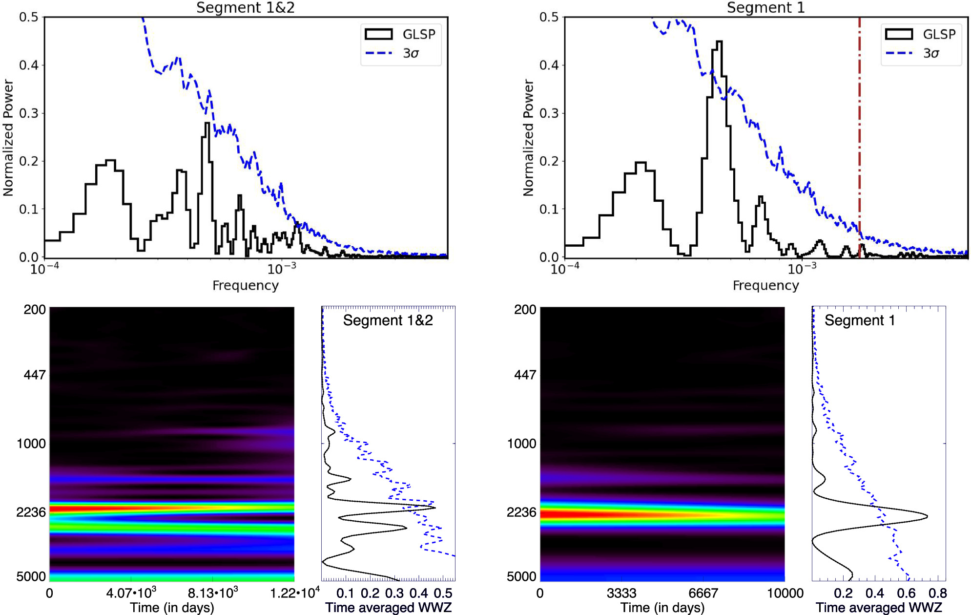
Figure 1 shows the LC of 3C 454.3 taken at 4.8 GHz in blue. The whole observation is divided into two segments. The second segment (after 2007) is dominated by flare features that we suggest originate from a process different from the stochastic processes that occurred in the first segment of the observation. To assess the effect of these flares on the variability exhibited by this source, we calculate the power spectrum for two cases: the whole LC (Segments 1 and 2) and Segment 1 alone. These are plotted in the upper panel of Figure 3. For the whole LC, a QPO signal at 0.00049 day−1, corresponding to around 2040 days, is found to be at least 3σ significant. For Segment 1, a QPO signal at a similar frequency (0.00045 day−1) is found at greater than 3σ significance. In the periodogram of the whole LC, there is one more peak adjacent to the claimed one, which is not present in the power spectrum of the first segment. This additional peak at lower frequencies appears to be contributed by the flares in Segment 2.

Figure 3. Upper panel: Generalized Lomb–Scargle periodogram for the whole light curve (left) and Segment 1 (right) at 4.8 GHz. The blue dashed curves respectively denote 3σ significance using a broken power law as the underlying red-noise model. Lower panel: Wavelet analysis for the entire light curve (left) and Segment 1 (right). In each panel, the left plot is the color–color diagram showing the WWZ power, where red denotes the most concentrated power, and the power decreases toward violet and black. The right plot shows the time-averaged WWZ along with 3σ significance given by the dashed blue curve.
Download figure:
Standard image High-resolution imageIn the bottom panel of Figure 3, WWZ power is plotted in the time–frequency plane for both the whole LC and just for Segment 1. In each case, the left panel shows the color–color diagram of WWZ power. For the whole LC, WWZ power is most concentrated at around 2080 days, and while it is persistent throughout the observation, it gets weaker during the last half of the entire span of the observations. As in the GLSP, there is a weaker signal centered at the frequency of 0.00038 day−1, which originates after the onset of the observations and continues until their conclusion. In Segment 1, the power is also concentrated around 2200 days, and this feature is more persistent in this segment than during the whole LC, and no weak feature is present around the lower frequency. The right panel shows the WWZ time-marginalized periodogram, which also indicates a significant oscillation at more than 3σ confidence.
The orange points in Figure 1 correspond to the LC collected at 8 GHz. The flare toward the end of the observation is even more significant than for the 4.8 GHz observation, but the other flux variations are very similar to those seen in the lower-frequency observations. The upper panel of Figure 4 shows the power spectrum analysis. For the whole LC, a signal at the frequency of ∼0.00048 day−1 is found to exceed 3σ significance using a simple power law. There are other peaks at higher frequencies, but none are significant. In the wavelet plot for the whole LC, a signal exceeding 3σ in the time-averaged WWZ is observed to be strong at the beginning of the observation, but it weakens toward the end of the observations. We see that the strong signal appears to bifurcate around the middle of the observations and eventually becomes two weaker signals. This could be the result of the flaring activity at the end of observation. When only Segment 1 of the LC is analyzed, the QPO peak at ∼0.00048 day−1 is stronger than that seen during the entire LC, exceeding 3σ regardless of the background model. In the wavelet plot, there is only one strong signal present, centered at 2380 days.

Figure 4. As in Figure 3 for the 8 GHz light curve.
Download figure:
Standard image High-resolution imageFigures 1 and 5 show the 14.5 GHz LC (green) and the GLSP and WWZ analysis results for the whole LC and Segment 1, respectively. After early 2007, there is a clear indication of flaring activity, which has significantly higher flux relative to the earlier fluctuations and is also stronger compared to both the 4.8 and 8 GHz LCs. In the GLSP result for the whole LC, the signal around 2125 days (∼0.00047 day−1) is marginally consistent with 3σ significance. In the GLSP plot of Segment 1, there is only one strong peak with at least 3σ significance, which is slightly shifted to ∼0.00042 day−1. The wavelet plots show similar behaviors to those of the 8 GHz LC. The wavelet color–color diagram of the whole LC shows a strong peak in the beginning, which fades as it approaches the end of the observations. There is also a second peak of lesser significance. The WWZ plot of Segment 1 shows a strong signal around 2325 days, which persists throughout this extensive portion of the observations, although it does weaken with time.

Figure 5. As in Figure 3 for the 14.5 GHz light curve. The dashed–dotted brown line in the GLSP plot of Segment 1 marks the possible QPO period at around 600 days.
Download figure:
Standard image High-resolution imageThe 22 GHz radio LC of 3C 454.3 is shown in Figure 1 in red. At this frequency, the extended flare in Segment 2 is even more dominant. The fluxes in Segment 1 are similar to those at the lower radio frequencies, but they are significantly higher in Segment 2. The influence of these flares is easily seen in the periodogram plotted in the upper panel of Figure 6. In the PSD of the whole LC (left figure), the signal at the period of around 2080 days is found with the marginal 3σ significance. If this baseline is affected by some other processes, then it is difficult to determine the appropriate significance levels, as is shown later in Section 3.4 through simulations. In the case of Segment 1 (right figure), the peak at the frequency of 0.00048 day−1 (2200 days) is found to have at least 3σ significance.

Figure 6. As in Figure 3 for the 22 GHz light curve. The dashed–dotted brown line in the GLSP plot of Segment 1 marks the possible QPO period at around 600 days.
Download figure:
Standard image High-resolution imageIn the wavelet plot for the whole LC (bottom panel), the WWZ power is mostly concentrated at the frequency of ≈0.00048 day−1, similar to what is found in the GLSP analysis, with more than 3σ significance as indicated in the time-averaged WWZ plot. For Segment 1, most power is concentrated around 2200 days, as also found in the GLSP method. One difference from the lower-frequency data is that the WWZ for the entire LC has more power concentrated toward the end of the observation while the opposite is the case for Segment 1.
At 37 GHz, the very powerful late flare is the most evident feature in the LC that is shown in Figure 1 in violet. The count rate for Segment 2 is almost double that of Segment 1; however, the fluctuations seen at lower radio frequencies are still evident in Segment 1. In the upper panel of Figure 7, the periodogram is plotted for the whole LC and for Segment 1. Similar to 22 GHz, the "red-noise" level for the whole LC is unstable, which results in less confident determinations of the underlying power-law models. So, no peak in its periodogram is found that has 3σ significance. In the wavelet color density diagram, the greatest power is concentrated toward the end of observation at multiple periods, more than that for 22 GHz. Although the signal at 0.00046 day−1 has 3σ significance (as seen in the time-averaged WWZ plot), it is strong only in the first half of the observation after which it starts to weaken, and then, more power around that frequency can be seen at the end of the observation. For Segment 1, the signal at 0.00042 day−1 is persistent throughout the observation, and it exceeds 3σ. No additional signals at the end of the observation are seen in this plot.

Figure 7. As in Figure 3 for the 37 GHz light curve. The brown dotted–dashed line in the GLSP plot of Segment 1 marks the likely QPO at ∼600 days.
Download figure:
Standard image High-resolution imageTable 1 lists the best-fit parameters for the broken power laws used to fit the power spectra of the observations. For all the radio frequencies, the high-frequency index α is as steep or steeper than the typical value found for blazars when analyzing Segments 1 and 2 together, ranging between 1.9 and 4.5. However, when only Segment 1 is considered, for all radio bands, α is found to have values in the range 2–3, within errors. The values of the slopes of the lower-frequency portion of the PSD, β, are all between 0.4 and 1.2.
Table 1. Best-fit Parameters for the Broken Power Used to Fit the Light Curves Analyzed in This Work
| Frequency | Segment | νb (×10−4) | β | α | N | C |
|---|---|---|---|---|---|---|
| 4.8 | 1, 2 | 0.66 ± 0.08 | 0.83 ± 0.09 | 1.87 ± 0.21 | 0.032 ± 0.002 | 0.011 ± 0.001 |
| 1 | 0.1 ± 0.01 | 1.21 ± 0.14 | 1.73 ± 0.21 | 0.037 ± 0.04 | 0.011 ± 0.001 | |
| 8 | 1, 2 | 2.82 ± 0.23 | 0.81 ± 0.1 | 4.52 ± 0.32 | 0.08 ± 0.006 | 0.063 ± 0.005 |
| 1 | 1.62 ± 0.13 | 0.97 ± 0.08 | 3.4 ± 0.43 | 0.078 ± 0.09 | 0.033 ± 0.004 | |
| 14 | 1, 2 | 3.3 ± 0.34 | 0.72 ± 0.08 | 4.02 ± 0.39 | 0.48 ± 0.054 | 0.066 ± 0.006 |
| 1 | 2.21 ± 0.24 | 0.52 ± 0.06 | 2.83 ± 0.31 | 0.99 ± 0.11 | 0.034 ± 0.003 | |
| 22 | 1, 2 | 3.9 ± 0.38 | 0.59 ± 0.06 | 4.23 ± 0.23 | 2.37 ± 0.22 | 0.406 ± 0.008 |
| 1 | 4.9 ± 0.05 | 1.21 ± 0.13 | 2.08 ± 0.20 | 0.002 ± 0.001 | 0.070 ± 0.007 | |
| 37 | 1, 2 | 2.03 ± 0.19 | 1.24 ± 0.11 | 2.61 ± 0.25 | 0.015 ± 0.002 | 0.316 ± 0.025 |
| 1 | 4.4 ± 0.04 | 0.35 ± 0.03 | 2.51 ± 0.28 | 3.093 ± 0.03 | 0.292 ± 0.034 | |
Download table as: ASCIITypeset image
3.2. A ≈600 Day Signal
Interestingly, a signal at around 600 days is also detected in these radio observations, but it is only significant in the LCs measured at higher radio frequencies. This apparent QPO is also suppressed by the flaring processes that began after early 2007. At 4.8 GHz, a peak at around 600 days is found in the GLSP result of the combined Segments 1 and 2, but it is not significant. This result also holds when only Segment 1 is analyzed. As this feature was not detected in the WWZ analysis, we do not claim it is present at this radio frequency. The same result also holds for the 8 GHz radio LC.
Table 2. Likely QPO Periods for Different Radio Frequencies Measured by Different Methods
| Frequency | Method | Segments 1 and 2 | Segment 1 |
|---|---|---|---|
| (GHz) | |||
| 4.8 | GLSP | 2093 ± 52 | 2272 ± 62 |
| WWZ | 2083 ± 26 | 2223 ± 52 | |
| 8 | GLSP | 2089 ± 30 | 2367 ± 70 |
| WWZ | 2127 ± 55 | 2380 ± 60 | |
| 14.5 | GLSP | 2125 ± 27 | 2283 ± 56 |
| WWZ | 2127 ± 63 | 2325 ± 65 | |
| 22 | GLSP | 2085 ± 34 | 2260 ± 52 and 580 ± 34 |
| WWZ | 2083 ± 26 | 2127 ± 55 | |
| 37 | GLSP | 2043 ± 27 | 2426 ± 64 and 582 ± 32 |
| WWZ | 2174 ± 64 | 2439 ± 121 | |
Download table as: ASCIITypeset image
A possible signal, although with significance less than 3σ, is observed to emerge around 600 days in the Segment 1 LC at 14 GHz, which is marked with a brown dashed line in the GLSP plot in Figure 5. For 22 GHz, no significant signal around that period is observed when the entire observation is analyzed. However, when only Segment 1 is examined, the significance is nearly 3σ (see Figure 6), which is higher than that obtained for 14 GHz. While this signal is rather weak in the WWZ analysis spanning Segments 1 and 2, it is clearly seen in the wavelet plot in Figure 6 for Segment 1. It persists throughout this portion of the observations and becomes stronger toward the end of it. The time-averaged WWZ signal reaches a 3σ significance. We conclude this feature was suppressed by the flaring that became dominant after 2007.
At 37 GHz, this feature at around 600 days is absent in the periodogram of the full set of observations. Instead, a signal around 870 days is present and appears to be roughly 3σ significant. The ≈600 day signal can be observed in the wavelet plot for all the data, albeit below 3σ significance. However, the 600 day signal is seen in the GLSP plot of Segment 1 in Figure 7 with more than 3σ significance, which actually makes this signal the most significant one at this radio frequency. The wavelet plot of Segment 1 also shows this signal with a significance exceeding 3σ. This 600 day signal corresponds to around 15 cycles of observations in the data up to 2007, indicating it is a rather strong candidate QPO period, at least in the LCs at 22 and 37 GHz.
3.3. ZDCF
Figure 8 shows the ZDCF analysis of the LCs used in this work for Segment 1 (top) and Segment 2 (bottom). The 4.8 GHz radio LC is taken as the base LC with respect to which the cross correlation is calculated. In Segment 1, the autocorrelation of the 4.8 GHz radio LC with itself also illustrates the quasiperiodic patterns discussed above with the first peak (at nonzero lag) at around 2400 days, and a ZDCF value of 0.25. The maximum ZDCF values of the 4.8 and 8 GHz and 4.8 and 14.5 GHz cross correlations are 0.92 and 0.85, respectively, with negative lags, indicating that the 4.8 GHz LC lags behind those at the higher frequencies, by 331 and 472 days, respectively. The peak ZDCF values against 4.8 GHz are found to be smaller at 22 GHz (0.69) and 37 GHz (0.47), with respective negative lags of 1010 and 1162 days. The lower peak ZDCF values at 22.0 and 37.0 GHz could arise from the lower fluxes at those higher frequencies, along with the confounding effects of the ∼600 day QPO apparently present in them. Another possible reason for such behavior could be differences in the sizes of emission regions, which can be expected to be smaller at higher radio frequencies as well as the difference in opacity at different radio frequencies. This behavior is consistent with the classic van der Laan adiabatically expanding source model (H. van der Laan 1966). More plausibly, if the variable radio emission arises from instabilities that weaken as they propagate downstream in the jet, the lower-frequency emission, which arises farther downstream, would be both delayed and reduced in amplitude.

Figure 8. Cross correlations between the radio light curves in Segment 1 (pre 2007) and Segment 2 (post 2007).
Download figure:
Standard image High-resolution imageIn Segment 2, the maximum ZDCF value is very high for all radio frequencies, as might be expected when only one major and one minor flare are present in that interval. The lags at 8 and 14.5 GHz are nearly the same as in Segment 1, but those at 22 and 37 GHz are smaller, supporting the hypothesis that a different physical mechanism is responsible for the flares in Segment 2, which are strongest at the highest frequencies. It is also possible that the same physical mechanism produces these flares, but the location or physical parameters producing the synchrotron emission are different.
This increased flux in Segment 2 at high radio frequencies also could lead to masking of the probable ∼600 day quasiperiod, which could only be recovered when analyzing Segment 1 individually.
3.4. Caveats
In principle, the physical mechanism responsible for flaring could be different from the usual stochastic processes occurring in jets or accretion disks of blazars that produce the run-of-the-mill variability. If this is the case, it would not be modeled appropriately with a (broken) power law, as is done for stochastic processes. Also, the statistical properties of the LC are different during flare and nonflare periods (P. Mohan et al. 2015). In the previous section for estimating the significance of the claimed QPO signals found in the whole LC (Segments 1 and 2), we fit the periodogram of Segment 1 and 2 jointly by a broken power law and then simulate the LCs. In this section, we want to assess how the significance estimates are affected if we model Segment 1 and Segment 2 separately. To assess the effects of these issues on our results, we simulate the LCs in two pieces. In this work, we consider the whole 37 GHz radio LC as the input observation. The first is comprised of the stochastic process model with a broken power law obtained by fitting the LC of Segment 1 at 37 GHz. The second component considered the flares modeled in the same way as for the first component but obtained by fitting Segment 2. Modeling the flare itself is outside the scope of this work, so we chose the broken power law for consistency. Then, we combine these two segments in time to form a single LC. In this way, we simulate 10,000 LCs and follow the procedure described in the Section 2.1 to obtain the desired confidence regime.
We compare our results with the case where both Segment 1 and Segment 2 are fitted jointly with the underlying broken-power-law model. Figure 9 shows 1σ confidence regions for the power spectrum density obtained by simulating the LCs fitting Segment 1 and Segment 2 separately, which is denoted by the red curve. The blue region corresponds to the error region for the PSD obtained by fitting the LC with a single red-noise model throughout the observation. The error estimates for both cases are consistent with each other in the frequency range of 0.0003 day−1–0.0015 day−1. As the claimed QPOs are found at frequencies higher than 0.0004 day−1, this will have minimal impact on our calculations. At frequencies lower than 0.0003 day−1, the confidence regions are significantly different. The error in the case that includes flares is smaller compared to the case that excludes flares and is consistent with each other above a frequency of 0.0003 day−1. Thus, fitting flares as a different stochastic process in the significance estimation would overestimate the errors for temporal frequencies less than 0.0003 day−1 but should not affect the QPO signal analyzed in this work.

Figure 9. Power spectrum simulations illustrating the effect of flaring activity on the error estimation using broken power law as underlying red-noise models.
Download figure:
Standard image High-resolution image4. Continuous Autoregressive Moving Average Analyses
To go beyond the basic modeling of PSDs in terms of a broken power law, we have also performed continuous autoregressive moving average (CARMA) analyses on these radio LCs. This is a method to model the LCs directly in the time domain and hence is not affected by the spectral distortions as in the case of frequency-domain analyses (e.g., B. C. Kelly et al. 2014; V. P. Kasliwal et al. 2017). A CARMA(p, q) process is the solution of the set of stochastic differential equations where p and q respectively define the order of autoregression and moving-average processes. For a CARMA process to be stationary, it is necessary that q < p. The majority of the long-term variability of AGNs is thought to originate in the accretion disk of the system and in the outflows and jets, which interact with the surrounding matter, and thus, there is a substantial possibility that the observed variability becomes complex and nonlinear in nature. Hence, fitting the observations with differential nonlinear equations of nth order should provide a better mode for such nonlinear processes.
We modeled the LCs analyzed in this work using CARMA(p, q) as implemented in the Eztao Python package (W. Yu et al. 2022), where 0 ≤ p ≤ 7 and 0 ≤ q < p. We fit each LC with CARMA models with different values of p and q and then select the model for which the Akaike information criterion is minimized. We then use that CARMA model to construct the periodogram and compare it with the Lomb–Scargle for a reality check. Figure 10 shows the PSD constructed using the best-fit CARMA model (written in the plot) and also the binned LSP. The CARMA derived PSDs all show their highest normalized powers around 0.00038 day−1 for all five radio frequencies, which is consistent with the QPO frequency claimed in this work.

Figure 10. The best-fit CARMA model PSD and binned Lomb–Scargle periodogram for the light curves at 4.8, 8.0, 14.5, 22.0, and 37.0 GHz. The Lomb–Scargle periodogram is plotted for comparison. The brown dashed curve denotes the frequency at which the highest value of normalized power is detected.
Download figure:
Standard image High-resolution image5. Discussion and Conclusions
In this work, we analyzed ≈35 yr long observations of a blazar 3C 454.3 taken at the radio frequencies of 4.8, 8.0, 14.5, 22.0, and 37.0 GHz where the flux density at 4.8, 8.0, and 14.5 GHz are obtained from UMRAO, and those at 22.0 and 37.0 GHz are from RT-22 and Aalto University Metsähovi Radio Observatory. The possible periodic modulations in flux can be seen in the LCs as shown in Figure 1. GLSP and WWZ methods are used to assess the periodicity observed in these LCs. To calculate the desired significance level, the power spectrum at lower frequencies is modeled with red noise, which means the power is inversely proportional to the frequency raised to some power. We used a broken power law to model the underlying red-noise stochastic process. Before 2007, the variability follows a stochastic process with an overlying QPO. After 2007, the LCs are dominated by a strong flaring process that is more significant at higher radio frequencies. We analyzed the observations with and without including this flaring period.
A period of around 2000 days is detected at all five radio frequencies, irrespective of the inclusion of the later flaring period in our analysis. Table 2 lists the probable QPO periods found using GLSP and WWZ analysis methods for these radio frequencies. The detection is considered strong if it is of at least 3σ significance in both the GLSP and the time-averaged WWZ analyses using a broken power law as the underlying red-noise model. For full LCs, this period corresponds to ≈6 putative cycles with 12,000 days as the temporal baseline of these observations. The strength of this signal increases at all the radio frequencies when the strong flaring period of Segment 2 is not included in the analysis, which suggests that this additional flaring activity makes a large change to the stochastic process and destroys or swamps any QPO. This effect can also be detected in the WWZ color diagram where most of the power is concentrated at the end of the observation when including the flaring period, and the diagram becomes chaotic as one examines the higher radio frequency LCs.
Interestingly, a quasiperiod of ∼600 days is also observed with at least 3σ significance at the frequencies of 22.0 and 37.0 GHz when the flaring period is excluded from the analysis. This period is also present in observation at lower radio frequencies but with less significance. This period corresponds to ≈16 putative cycles of observations. As the claimed quasiperiodic frequencies are more than 0.0003 day−1, the error estimates on the periodogram are not affected by the flaring processes significantly, which was shown through simulations discussed in Section 3.4.
In blazars, the nonthermal emission from jets and accretion disks dominates the cumulative emission in all EM bands. Time-dependent changes in the fueling of the jet by the central engine (BH plus accretion disk) would affect the development and growth of the instabilities in the jets. And the origin of the emission at the radio frequencies employed in this work certainly comes from the jet, which is strongly Doppler boosted owing to its low inclination angle (∼1 3; T. Hovatta et al. 2009). Therefore, any quasiperiodicity observed is much more likely to be the result of internal jet processes than processes in the accretion disk.
One likely origin of these long-period QPOs is the presence of a binary SMBH system, as is almost certainly present in OJ 287 (see H. J. Lehto & M. J. Valtonen 1996; A. Sillanpää et al. 1996; J. H. Fan et al. 2007; S. Britzen et al. 2017; E. Kun et al. 2018; A. C. Gupta et al. 2023; M. J. Valtonen et al. 2024, and references therein). In this now standard model for OJ 287, flares are produced when the secondary BH smashes through the accretion disk around the primary. Alternatively, in a binary model, the accretion rate onto one BH can increase significantly when the other one comes in its proximity due to an elliptical orbit even if it does not impinge upon the disk. This increase in accretion rate could lead to the periodic increase in the flux (G. G. Wang et al. 2022). However, this model would be more important when the emission from the accretion disk exceeds that from the jet, which is unlikely in the case of blazars and particularly unlikely for radio emission. The orbital motion of the two BHs can naturally yield periodic fluctuations in observed radio flux from the change in Doppler factor caused by variation in the observation angle to the jet (e.g., M. Villata et al. 2006; S.-J. Qian et al. 2007). Recently, S. O'Neill et al. (2022) applied this model to explain the quasiperiodicity of ∼1700 days in the blazar PKS 2131−021. So, the binary SMBH hypothesis provides a plausible explanation for the ∼2000 day QPO supported by our analysis.
The wiggling of the jet could also be produced internally via Lens–Thirring precession occurring in the inner part of the accretion disk, from which the jet is presumably launched, due to relativistic frame-dragging (L. Stella & M. Vietri 1998; M. Liska et al. 2018). The Lens–Thirring precession model more naturally produces periodicity of the order of a few months. So, while this model is unlikely to explain the ∼2000 day QPO, it might produce the putative ∼600 day one, which is apparently detected in the LCs at higher radio frequencies (22.0 and 37.0 GHz). While it also may be present at the lower frequencies, the broader peaks at lower frequencies could make it harder to detect.
Another possible explanation of these QPOs is related to the internal helical structure in the jet (see F. M. Rieger 2004; P. Mohan & A. Mangalam 2015, and references therein). In this model, shocks generated in current-driven plasma are believed to propagate outwards toward the jets and interact with the toroidal magnetic field of the jet, leading to its distortion. These sudden changes affect the magnetic fields around the BH and result in the periodic fluctuations manifested in the observed flux from the jet (e.g., M. Camenzind & M. Krockenberger 1992; L.-X. Li & R. Narayan 2004). These periodic changes occur on the order of a few months to years and so could explain either the observed 2000 day QPO or the possible 600 day periodicity seen in this work. Magnetohydrodynamic simulations suggest that some QPOs could be the result of quasiperiodic kinks arising in the jet due to the instability produced by distorted magnetic fields (e.g., J. C. McKinney et al. 2012; L. Dong et al. 2020). However, if these fluctuations are due to kink instabilities, they would be by far the longest discovered so far, as kink-driven oscillations seem to persist for only days or weeks (e.g., S. G. Jorstad et al. 2022; A. Tripathi et al. 2024a, 2024b).
Figure 11 shows a series of SEDs where the flux densities at all five radio frequencies are plotted at different times. The left plot shows the SEDs during Segment 1, and the right plot shows the SEDs during Segment 2. In Segment 1, the flux density usually declines monotonically with frequency, as is typical for radio synchrotron emission from a steady jet. But during the high emission states in 1982.0 and 1994.5, the flux density peaks around 8 GHz. During these epochs, the highest frequency emissions are past their peaks and already fading; those around 8 GHz are near their peaks, while at 4.8 GHz the flux is still rising. This can be understood if emission at lower frequencies is delayed and is broadened as it emerges from a larger region. This behavior of flux variation at different radio frequencies is expected with the standard shock-in-jet model (e.g., A. P. Marscher & W. K. Gear 1985; P. A. Hughes et al. 1989).

Figure 11. Spectral energy distributions (SEDs) plotted at all five radio frequencies analyzed in this work. The left panel shows the SEDs during Segment 1, and the right panel shows the SEDs during Segment 2.
Download figure:
Standard image High-resolution image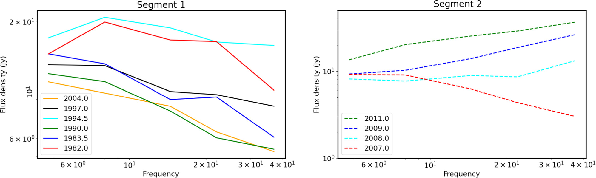
However, in Segment 2, the behavior of the SEDs is generally very different. At the beginning of this period at 2007.0, when the source is dim, there is a continuation of the usual essentially monotonic decline of flux density with frequency. Afterward, when the flaring process dominates, the SEDs shift toward a trend of increasing flux with rising frequency. This behavior of the SEDs indicates that the physical process governing the strong flares in Segment 2 (2007 onwards) may be different from that of Segment 1. A likely scenario would be the presence of a knot emerging from the core and passing through the standing shock in the jet, as depicted in the VLBI image of 3C 454.3 at 43 GHz (A. P. Marscher et al. 2008). Such behavior, known as core-shift variability, has also been found in the VLBI images at different radio frequencies made between 2005 and 2010 (W. Chamani et al. 2023), during the flares seen in Segment 2. S. G. Jorstad et al. (2010) analyzed multifrequency LCs of this object during 2005–2008 as well as Very Long Baseline Array maps they made at frequent intervals and concluded that the variability predominantly arises from outward moving knots interacting with a stationary knot in the jet ∼0.6 mas from the core. Recently, E. Traianou et al. (2024) analyzed VLBI images at 43 and 86 GHz of this source during 2013–2017 and found that some superluminal features abruptly disappeared at that stationary knot. They claimed that these peculiar kinematics can be explained by the presence of a bend in the jet at that characteristic location.
One interesting result of this work is the discovery of an apparent ∼600 day signal, which is most prominent at higher frequencies. This signal becomes strong toward the middle of the observations and persists until the end of the observations of Segment 1. However, the flaring seen in Segment 2 apparently suppresses this signal.
Acknowledgments
This work is supported by NASA grant No. 80NSSC22K0741. This research is based on data from the University of Michigan Radio Astronomy Observatory, which was supported by the National Science Foundation, NASA, and the University of Michigan. UMRAO research was supported in part by a series of grants from the NSF (including AST-0607523 and AST-2407604) and by a series of grants from NASA, including Fermi G.I. awards NNX09AU16G, NNX10AP16G, NNX11AO13G, and NNX13AP18G. This publication makes use of data obtained at Metsähovi Radio Observatory, operated by Aalto University in Finland. The various diligent observers of Aalto University are thankfully acknowledged.
Footnotes
- 10
- 11
- 12