


Abstract
The microphysics of the intracluster medium (ICM) in galaxy clusters is still poorly understood. Observational evidence suggests that the effective viscosity is suppressed by plasma instabilities that reduce the mean free path of particles. Measuring the effective viscosity of the ICM is crucial to understanding the processes that govern its physics on small scales. The trails of ionized interstellar medium left behind by the so-called jellyfish galaxies can trace the turbulent motions of the surrounding ICM and constrain its local viscosity. We present the results of a systematic analysis of the velocity structure function (VSF) of the Hα line for ten galaxies from the GASP sample. The VSFs show a sublinear power-law scaling below 10 kpc that may result from turbulent cascading and extends to 1 kpc, which is below the supposed ICM dissipation scales of tens of kpc expected in a fluid described by Coulomb collisions. Our result constrains the local ICM viscosity to be 0.3%–25% of the expected Spitzer value. Our findings demonstrate that either the ICM particles have a smaller mean free path than expected in a regime defined by Coulomb collisions or that we are probing effects due to collisionless physics in the ICM turbulence.

Original content from this work may be used under the terms of the Creative Commons Attribution 4.0 licence. Any further distribution of this work must maintain attribution to the author(s) and the title of the work, journal citation and DOI.
1. Introduction
The intracluster medium (ICM) microphysics in galaxy clusters is poorly known. It is usually assumed to be a fluid dominated by Coulomb collisions, which can explain its large-scale properties (e.g., C. L. Sarazin 1988). However, the properties of the gas density fluctuations (I. Zhuravleva et al. 2019) and the observational evidence of cosmic ray electron reaccelerated by ICM turbulence (e.g., G. Brunetti & T. W. Jones 2014) indicate that the effective ICM viscosity is orders of magnitude smaller than expected from the thermal ion–ion Coulomb collisions (e.g., L. Spitzer 1962). This is because the ICM is a "weakly collisional" plasma due to various plasma instabilities, (e.g., A. A. Schekochihin 2022, for a review) that can perturb the ICM magnetic field on small scales, thus strongly reducing the effective ICM particles' mean free path, and hence also the effective viscosity of the fluid.
Cluster galaxies can be used to probe the ICM properties, especially the so-called jellyfish galaxies (e.g., R. J. Smith et al. 2010; H. Ebeling et al. 2014; M. Fumagalli et al. 2014; B. M. Poggianti et al. 2017a; A. Boselli et al. 2022) that are the result of infalling spiral galaxies interacting with the ICM. These galaxies show characteristic "tails" of ionized plasma that is produced by the interstellar medium (ISM) being displaced outside of the stellar disk via ram pressure stripping (RPS; J. E. Gunn 1972), where the ISM and the ICM can interact via mixing. Observational evidence of ISM–ICM mixing has been collected in various forms, from metallicity gradients along the tails (A. Franchetto et al. 2021), to extended X-ray emission associated with the Hα emission (e.g., M. Sun et al. 2010, 2021; B. M. Poggianti et al. 2019a; M. G. Campitiello et al. 2021; C. Bartolini et al. 2022), to peculiar optical line ratios (B. M. Poggianti et al. 2019b; M. G. Campitiello et al. 2021), to the presence of diffuse ionized gas (N. Tomičić et al. 2021; A. Pedrini et al. 2022), or large-scale magnetic fields accreted from the ICM (A. Müller et al. 2021). All these results point toward the fact that in the tails of jellyfish galaxies the stripped ISM dynamic is affected by the ICM small-scale motions, such as turbulence. Therefore, the diffuse ISM Hα emission might probe the ICM turbulent motions, and thus trace the turbulent cascade down to its dissipation scale, hence constraining the ICM viscosity. Y. Li et al. (2023) pioneered this method by analyzing the velocity structure function (VSF) in the tail of the nearby jellyfish galaxy ESO137-001. The VSF is a two-point correlation function that quantifies the kinetic energy fluctuations as a function of the scale l in a velocity field. The VSF can trace both the energy cascade expected in turbulent flows and coherent motions, such as collapse, rotation, or blast waves, which appear in the form of coherent velocity differences (e.g., A. Kolmogorov 1941; M. H. Heyer & C. M. Brunt 2004; R. A. Chira et al. 2019). For fluid particles in fully developed, homogeneous, and isotropic turbulence, A. Kolmogorov (1941) predicted that the VSF is well described by a power-law relation that extends down to a dissipation scale, η, which depends on the fluid viscosity. Y. Li et al. (2023) observed a turbulent cascade in the VSF of ESO137-001 extending for two orders of magnitude below the supposed dissipation scale, thus constraining the ICM viscosity to ∼0.01 of the predicted value.
In this paper, we extend the VSF analysis to a sample of 10 galaxies from the GASP survey 9 (GAs Stripping Phenomena in galaxies with MUSE, B. M. Poggianti et al. 2017a). By operating on a larger sample, we can simultaneously test the results of Y. Li et al. (2023) and explore the variation in ICM viscosity for different galaxy cluster properties and regions. This paper is structured as follows. In Section 2, we present the sample and the data preparation, from MUSE data processing to the VSF construction. In Section 3, we report and discuss the results, and in Section 4 we list the main caveats of our analysis. Finally, in Appendices A and B we report a series of diagnostic plots, in Appendix C, we show the VSF for the entire sample and in Appendix D we describe the simulation setup adopted to compare the observed VSFs. In this work we adopt the standard concordance cosmology parameters H0 = 70 km s−1 Mpc−1, ΩM = 0.3, and ΩΛ = 0.7. At the redshifts of the clusters in which galaxies are located, 1'' ≃ 0.9–1.1 kpc.
2. Data Analysis
2.1. Sample Selection
To investigate the properties of the stripped ISM, we select the most extreme ram pressure stripped galaxies from the GASP sample, which is composed of galaxies at z = 0.04–0.07 located in different environments, from the field to clusters. Specifically, we select the 10 galaxies in clusters with the most extended Hα tails in the plane of the sky in the MUSE images. Their properties, and those of their hosting clusters, which are presented in B. M. Poggianti et al. (2017a) and M. Gullieuszik et al. (2020), are summarized in Table 1. The resulting sample spans more than two orders of magnitude in stellar mass, from log (Mstar/M⊙) = 9.05 (JW56) to log (Mstar/M⊙) = 11.47 (JW100) and covers different regions in the phase-space diagram (Figure 1), which indicates that galaxies are in different ICM and RPS conditions.
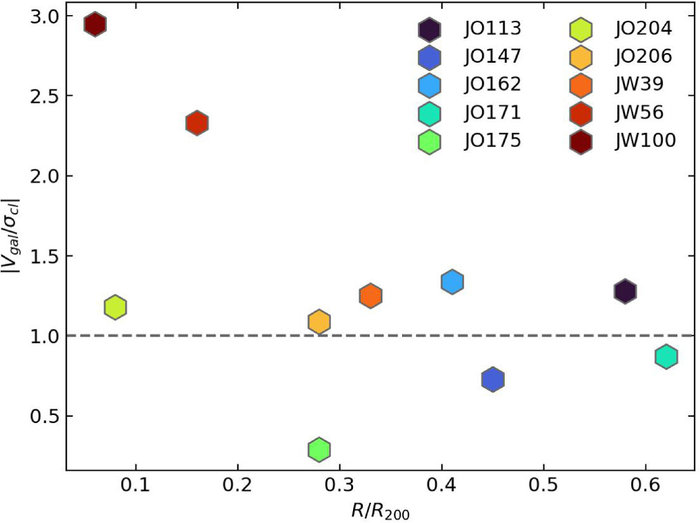
Figure 1. Line-of-sight velocity in units of the hosting cluster velocity dispersion vs. projected position in units of R200. The horizontal dashed line indicates ∣Vgal∣ = σcl.
Download figure:
Standard image High-resolution imageTable 1. Sample Properties
| Galaxy | zgal | log Mstar/M⊙ | Cluster | zcl | log M200/M⊙ | R200 | σcl | Rgal/R200 | ∣Vlos/σ∣ |
|---|---|---|---|---|---|---|---|---|---|
| (Mpc) | (km s−1) | ||||||||
| JO113 | 0.0552 | 9.69 | A3158 | 0.05947 | 14.94 | 1.94 | 948 | 0.58 | 1.28 |
| JO147 | 0.0506 | 11.03 | A3558 | 0.04829 | 14.95 | 1.95 | 910 | 0.45 | 0.73 |
| JO162 | 0.0454 | 9.42 | A3560 | 0.04917 | 14.83 | 1.79 | 799 | 0.41 | 1.34 |
| JO171 | 0.0521 | 10.61 | A3667 | 0.05528 | 15.12 | 2.22 | 1031 | 0.62 | 0.87 |
| JO175 | 0.0467 | 10.50 | A3716 | 0.04599 | 14.78 | 1.72 | 753 | 0.28 | 0.29 |
| JO204 | 0.0424 | 10.50 | A957 | 0.04496 | 14.53 | 1.42 | 631 | 0.08 | 1.18 |
| JO206 | 0.0511 | 10.96 | IIZW108 | 0.04889 | 14.31 | 1.20 | 575 | 0.28 | 1.09 |
| JW39 | 0.0663 | 11.21 | A1668 | 0.0634 | 14.48 | 1.35 | 654 | 0.33 | 1.25 |
| JW56 | 0.0387 | 9.05 | A1736 | 0.0461 | 14.92 | 1.92 | 918 | 0.16 | 2.33 |
| JW100 | 0.0619 | 11.47 | A2626 | 0.05509 | 14.59 | 1.48 | 650 | 0.06 | 2.95 |
Note. From left to right: GASP name; Galaxy redshift; Stellar mass; Hosting cluster name, redshift, M200, R200, and velocity dispersion σcl (B. Vulcani et al. 2018; M. Gullieuszik et al. 2020); Galaxy cluster-centric distance in units of R200; Galaxy velocity along the line of sight in units of σcl.
Download table as: ASCIITypeset image
These galaxies, and their stripped tails, have been the subject of previous studies. They all show Hα tails with projected lengths of a few tens of kpc that host extraplanar star formation (B. M. Poggianti et al. 2019b; N. Tomičić et al. 2021). In the MUSE spectra, JW56 and JW100 show extended regions in which the optical line ratios are consistent with LINERS emission (B. M. Poggianti et al. 2019b), indicating that the main ionization mechanism could be the photoionization due to the ICM thermal emission (M. G. Campitiello et al. 2021). For JW100, Chandra observations detected extended X-ray emission in the tail, which correlates spatially with the Hα emission (B. M. Poggianti et al. 2019a) and supports the hypothesis of ongoing ISM–ICM mixing (M. Sun et al. 2021). Finally, in JO206, JW39 and JW100 show nonthermal radio tails (A. Müller et al. 2021; A. Ignesti et al. 2022a), which is evidence of large-scale magnetic fields extending in the tails.
2.2. MUSE Data Preparation
This work is based on the kinematics of the ionized gas derived from the Hα emission. We use the MUSE data from the GASP survey; the observations, data reduction, and analysis are presented in B. M. Poggianti et al. (2017a). The spatial resolution of these seeing-limited observations is ∼1'', which at the redshift of the targets corresponds to ∼1 kpc. Emission line fluxes and gas kinematics were measured using the IDL software KUBEVIZ (M. Fossati et al. 2016) on the data cubes obtained by subtracting the stellar component from the observed data and corrected for dust extinction (for details see B. M. Poggianti et al. 2017a). KUBEVIZ also provides the 1σ error for each fitted parameter, including the line-of-sight velocity. We report the Hα line velocity maps in the galaxy rest-frame by normalizing them for the average velocity measured at the center of the stellar disk.
2.3. Velocity Structure Function
The stripped tails are complex, filamentary structures in which the properties of the plasma are affected by the presence of star-forming complexes (B. M. Poggianti et al. 2019b; E. Giunchi et al. 2023), and by other large-scale dynamical processes which imprint coherent velocity differences in the VSF. Thus, it is necessary to further process the data to recover the turbulence signature in the Hα VSF.
2.3.1. Step I: Locating the Diffuse ISM
We first filter the data to extract only the signal from the extraplanar diffuse emission. Specifically, the spaxels of the tails from which to measure the line velocity are selected by applying a series of filters in the Hα images. To begin with, we consider only those pixels with a signal-to-noise ratio higher than 5 in the Hα flux density, with a flux density lower than 10−16 erg s−1 cm−2, to avoid hot pixels, and with an uncertainty on the velocity fit lower than 30 km s−1. Moreover, we mask the pixels located inside of the stellar disk (as defined in M. Gullieuszik et al. 2020) and the star-forming clumps detected in Hα (B. M. Poggianti et al. 2017b). This latter condition is physically motivated by the consideration that the plasma in the clumps which surrounds the new stars is less likely to be bound to the turbulent ICM. This selection provides us with the signal from the extraplanar, diffuse plasma in the tails. From the remaining signal, we further remove the isolated regions with an area smaller than 200 pixels for which it is difficult to ascertain that they really belong to the stripped tails.
2.3.2. Step II: Filtering Out Rotation and Advection
The stripped ISM dynamic outside the stellar disk is primarily set by the combination of (1) advection induced by the ram pressure, (2) rotation inherited from the disk, and (3) ISM small-scale motions (e.g., M. Gullieuszik et al. 2017; S. Tonnesen & G. L. Bryan 2021; N. Akerman et al. 2023; R. Luo et al. 2023; M. Sparre et al. 2024). To study the ISM small-scale motions, and hence the ICM turbulence signature in the VSF, it is crucial to remove the other two factors. However, their removal is complicated by the intrinsic filamentary structure of the stripped ISM, which makes it difficult to define an unambiguous rotation axis to conduct an analysis of the 3D rotation (e.g., C. Bacchini et al. 2023, for the analysis of the rotating molecular gas in the disks of the same GASP galaxies), and by projection effects, which can lead gas originating from different sides of the disk to overlap along the line of sight. Therefore, we propose a novel technique to remove these components from the velocity field, which we show here for JO206, and for the other galaxies in Appendices A and B.
To visualize the structure of the velocity maps, we compose the phase-space diagram for each galaxy, where we compare the velocity measured in each pixel with its minimum distance from the stellar disk edge, as defined in M. Gullieuszik et al. (2020). The diagrams are then converted into density plots to highlight the substructures in the velocity maps (Figure 2, top panel). First, we correct the velocity field for the advection component along the line of sight. The ram pressure can induce a velocity increase with the distance from the stellar disk as the gas clouds gradually approach the ICM wind speed (R. Luo et al. 2023; P. Serra et al. 2023). So, we compute the median velocities at increasing distances from the disk and use them to fit a linear model of the velocity gradient along the tail (Figure 2, top panel, orange points). Then, we subtract this systematic component from each pixel depending on their distance from the disk. A similar procedure is presented also by R. Luo et al. (2023) to correct the systematic velocity in ESO137-001. This correction can also remove the systematic velocity shift derived from the galaxy velocity in the cluster. The result is a velocity distribution that is typically centered around zero without clear gradients with the distance (Figure 2, central panel). However, we recognize the presence of clear filamentary patterns in the residual phase-space intensity distribution. We assume that these structures are produced by the rotation of the stripped gas inherited from the disk kinematics.

Figure 2. Phase-space density plots derived from the Hα velocity map of JO206. Top panel: Initial velocity distribution with the median velocities (orange points) and the best-fitting velocity gradient. Central panel: Velocity distribution corrected for the systematic velocity. The colored points trace the rotating filaments, and the lines point out the corresponding average velocity. Bottom panel: Resulting velocity distribution corrected for the rotation of each filament.
Download figure:
Standard image High-resolution imageTo remove the rotation, we first identify the different filaments in the phase-space density plots as regions where the points are clustered around certain velocity values. To do so, we bin the phase-space plots in several velocity bins and then for each bin we compute the median velocity values at increasing distances from the disk. The numbers of velocity and distance bins are different for each galaxy and they are set by visual inspection. For each filament (colored points in Figure 2, central panel), we compute the average velocity, weighted by the number of points in each bin (colored lines in Figure 2, central panel). Then, we correct each filament by subtracting the corresponding average velocity from each pixel in their bins. At this step, we mask out those pixels located outside the filaments. This operation independently corrects each filament for its velocity, resulting in a velocity distribution centered around zero and without any clear symmetric structure (Figure 2, bottom panel). Finally, we further mask out the strong outliers, which typically are residuals left by rotation correction or contaminations from the [N ii] line. In Figure 3, we show the original velocity map of the diffuse, stripped ISM (top panel) and the model obtained by combining the advection and rotation components (bottom panel).

Figure 3. Hα observed (top panel) and rotation+advection model (bottom panel) velocity map of JO206. We also show the original Hα emission (gray colormap), and the stellar disk (gray contour, M. Gullieuszik et al. 2020).
Download figure:
Standard image High-resolution image2.3.3. Step III: Computing the VSF
The VSFs are computed from the pixels of the residual velocity map as follows: for each pair of pixels, we measure their projected physical distance l, which we derive by multiplying their angular separation by the kpc-to-arcsec scale at the hosting cluster redshift, and the velocity difference δ V. The VSF is derived by computing the average absolute value of the velocity differences 〈∣δ V∣〉 within bins of l from 0.2 to 100 kpc with a step of 0.2 kpc, which is approximately the physical scale corresponding to the pixel size of the MUSE images. Correspondingly, by propagating the uncertainties on the velocity measurement of each spaxel, the uncertainties on the fit of the systematic velocity, and the rotating filaments, we compute the error on each bin of the VSF that results in the order of a few km s−1. We show in Figure 4 the residual velocity map (left-hand panel) and the corresponding VSF (blue line). For comparison, we use the original velocity map not corrected for the rotation and advection to compute the VSF in the tail (VSFNC, orange-dashed line), and inside the stellar disk (VSFDisk, green-dashed–dotted line). The VSFs show different slopes, with the first one resembling the slope l1/3 (gray-dashed line), and the other ones being generally steeper and more similar to the linear scaling (black line). We note that as a consequence of atmospheric seeing the effective angular resolution is limited to ∼1'' (≃1 kpc marked in gray in Figure 4), and thus below that scale the VSF signal is less reliable because the pixels are correlated within the resolution elements. Therefore, in the following analysis we conservatively consider l = 1 kpc as the lower limits of the VSFs. As a caveat, it is important to remember that this analysis is subject to projection effects because filaments that are physically distant can appear adjacent along the line of sight. We refer to Section 4 for a detailed discussion of the role of projection effects.

Figure 4. Left-hand panel: Residual velocity map of JO206 (blue-to-red colormap). We also show the original Hα emission (gray colormap) and the stellar disk (gray contour, M. Gullieuszik et al. 2020). Right-hand panel: VSF of the residual velocity map (blue, the blue-filled area indicates the 1σ uncertainty region), the one derived from the not-corrected one (orange), and the one derived in the stellar disk only (green). The gray-shaded area marks l < 1'', below which the signal is affected by the spaxel correlation (see Section 2.2). The continuous and dashed lines indicate the slopes expected in the case of, respectively, rotation (∝l) and turbulence (∝l1/3).
Download figure:
Standard image High-resolution image2.4. Comparison with a Simulated Case
To further corroborate our analysis, we explore the case of the VSF in the absence of ICM turbulence. To do so, we make use of the simulation setup presented in N. Akerman et al. (2023) (see Appendix D). The simulation models stripping of a massive Milky Way-like galaxy with a radius of ∼30 kpc and which rotates at ∼200 km s−1. In this set-up, the gas dynamics are set solely by rotation and ram pressure, and the simulated ICM wind is initially laminar at the galaxy scale. Furthermore, there are no magnetic fields. We produced maps of the gas velocity along the line of sight for the gas phase in the temperature interval 3.5 < logT <6.5, each one at four different snapshots in time (100, 200, 300, and 400 Myr after the beginning of the stripping). The maps capture the gas in the stripped tails, defined as 2 kpc above the galaxy plane in the direction of stripping. Specifically, we analyze the case of face-on stripping (W0) and inclined stripping (W45, wind hits the galaxy at 45°). In W0, the wind blows along the z-axis, while in W45 the wind has components along both the y- and the z-axes. The latter ensures that the line of sight is aligned with the stripping direction and allows us to further investigate the role of projection effects. For the simulated VSFs, we take the gas projections along the x-axis for both W0 and W45 galaxies, and an additional projection along the y-axis for W45 ("W45-y" in Figure 5). We set the pixel size of the velocity maps to 0.2 kpc to match the physical scale of the MUSE images. The VSFs are computed with the same method adopted for the real MUSE observations, i.e., by considering only the gas outside of the stellar disk. We note that at this stage we do not attempt to remove the rotation and advection. The resulting VSFs are shown in Figure 5, divided by simulation run (rows). The velocity maps themselves can be found in Appendix D.

Figure 5. VSFs of the simulated tail for different inclinations (top to bottom) at different snapshots. The VSFs reported here are derived without prior reprocessing of the simulated velocity maps. The continuous and dashed lines indicate the slopes expected in the case of, respectively, rotation (∝ l) and turbulence (∝ l1/3).
Download figure:
Standard image High-resolution imageIn the early stages (100–200 Myr), when the tail is still rich in rotating gas (see Figure 14), the VSFs show a recurrent shape characterized by an almost constant slope from 0.2 to 2–3 kpc, a strong inflection between 3 and 7 kpc, and linear slope expected by the rotation up to the disk radius scale. As a cautionary tale we note that for the late-stage stripping, when the tail has already lost most of the gas and what is left does not keep track of the disk rotation anymore, the VSFs are flatter than the initial-stage stripping case. This result suggests that an advection-dominated tail, in which the gas particles move with a uniform velocity set by the ram pressure wind, results in a sublinear VSF, which is similar to a turbulent-dominated one.
Finally, we use the simulated tails to demonstrate the effectiveness of the correction procedure described in Section 2.3.2. Specifically, we perform the procedure on the W45-y run, at 300 Myr after the beginning of the stripping because of the complex morphology composed of filamentary structures visually resembling the observed tails. We show each step and the final results in Figure 6. After the removal of rotation and advection, the residual VSF (blue line) results are significantly flattened, which denotes the fact that the residual velocity map is devoid of large-scale coherent velocity differences, thus confirming the efficacy of the procedure. We note that the residual VSF is also flatter than the turbulent slope, which indicates that the simulated tails lack small-scale turbulent motions. We conclude that this is likely due to the limits of the simulation setup (see Appendix D), which cannot fully resolve the turbulence development. Although done intentionally because such a configuration is designed to save on computational time and resources, and furthermore the simulation was designed for a different scientific analysis (see N. Akerman et al. 2023), this means that future studies aiming to focus on the development of stripped tails will require tailored numerical simulations.

Figure 6. Correction procedure applied on the simulated tail W45-y at 300 Myr after stripping. Left-hand panels: Phase-space density plot for the simulated tail; Middle panels: Comparison between the original (top panel), model (center panel), and residual (bottom panel) velocity maps; Right-hand panel: VSF before (orange) and after (blue) the correction procedure (Section 2.3.2). The continuous and dashed lines indicate the slopes expected in the case of, respectively, rotation (∝ l) and turbulence (∝ l1/3).
Download figure:
Standard image High-resolution image3. Results and Discussion
3.1. Results
In Figure 7, we show the resulting, corrected VSF for each galaxy compared with the Kolmogorov spectrum 〈∣δ V∣〉 ∝ l1/3 (A. Kolmogorov 1941). The individual VSFs are presented in Appendix C. Generally, the galaxies approximately follow the ∝l1/3 scaling below 5 kpc, whereas they are flat on larger scales due to the removal of rotation and advection, which dominate the large-scale dynamic. This pattern is consistent with the one shown by Y. Li et al. (2023).

Figure 7. Comparison of the VSF of the entire sample. The black-dashed line indicates the l1/3 trend. The gray-filled region marks l < 1'' below which the signal is affected by the spaxel correlation (See Section 2.2).
Download figure:
Standard image High-resolution imageThe residual VFSs are different from the simulated ones (Figure 5), lacking both the steep, high-velocity part at large scales, induced by the combination of rotation and advection, and the flattening at small scales. On the contrary, these features are present in the not-corrected VSFs (Appendix C, orange lines). Therefore, we argue that we have removed most of the rotation and advection components, and thus the residual VSFs trace the small-scale, turbulent motions of the stripped ISM.
3.2. What Drives the Turbulence in the Tails?
The turbulent cascade we observe could either result from the "frozen-in" ISM turbulence inherited from the disk or the ICM turbulence. To test the first scenario, in Figures 4 and 13 we compare the VSF computed inside (green lines) and outside (orange lines) of the stellar disk. We observe two cases, galaxies in which the disk VSF is lower than the tail one (JO113, JO162, JO175, JO206, and JW39), and galaxies in which we observe the opposite (JO147, JO171, JO204, JW56, and JW100). The first case naturally challenges the frozen-in ISM turbulence scenario because it indicates that the ISM turbulence can be weaker and the tail turbulence is likely dominated by the growth of instabilities induced by the interaction with the ICM. Regarding the second case, we observe that the ISM turbulence can be significantly strong (e.g., the case of JW56 and JW100), but once the gas is stripped it decays quickly. For JW56 and JW100, the flattening of the VSF takes place at the 2–3 kpc scale with δ v ∼ 70 km s−1. The driving scale is typically a factor 2–3 larger than the flattening scale (C. Zhang et al. 2024), thus we estimate an eddy turnover time (t ≃ l/v) of ∼50–100 Myr. Assuming an average stripped plasma velocity of 300 km s−1, which is in line with the constraints provided by the decay of the radio continuum emission in ram pressure stripped tails (A. Ignesti et al. 2023; I. D. Roberts et al. 2024), then within one eddy turnover time the stripped ISM has moved about ∼15–30 kpc. This length scale is consistent with the observed tail length. So, we argue that what we observe in the tail is never pure, frozen-in ISM turbulence but we are tracing fully mixed ISM or, at least, stripped ISM in a transition stage.
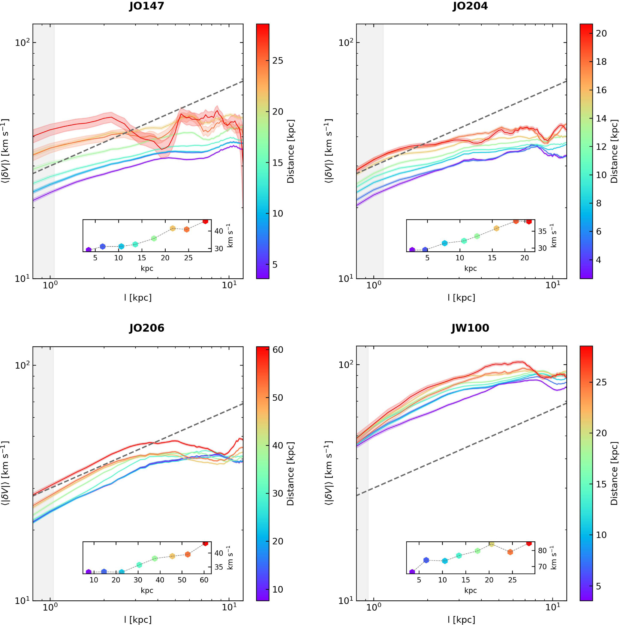
To further understand how turbulence develops in the tails of GASP galaxies, we study the variation of the residual VSF at increasing distances from the stellar disk. We perform this analysis on JO147, JO204, JO206, and JW100, the galaxies with the longest tails in the sample. Similar to the approach presented by Y. Li et al. (2023), we define an adaptive moving frame, with a width corresponding to one-third of the tail length, in which we compute the VSF in eight bins at increasing distance from the stellar disk. We also compute the average value of each VSF between 2 and 3 kpc to quantify the trend with the distance. The results are shown in Figure 8.

Figure 8. VSFs at increasing distance from the disk for JO147, JO204, JO206, and JW100. The VSFs are computed within a moving frame along the tail direction, color-coded by the distance of the frame center from the stellar disk edge. The dashed line indicates the Kolmogorov slope. In the inserts, we report the average VSF value between 2 and 3 kpc at increasing distances from the disk.
Download figure:
Standard image High-resolution imageThe resulting VSFs broadly follow the l1/3 slope below 5 kpc, as Figure 7 shows. We observe a gradient with the distance, with the farthest bins showing a higher level of turbulence with respect to those close to the disk. This result is in line with a scenario where the mixing with the ICM is increasing the stripped ISM turbulence velocity with respect to the initial stellar disk conditions (F. Fraternali et al. 2002; G. Iorio et al. 2017; C. Bacchini et al. 2020). Therefore, the observed VSFs support our hypothesis that environmental turbulence ultimately drives the stripped gas small-scale motions.
3.3. Implications for the ICM Microphysics
Our working hypothesis, based on the observational evidence of ISM–ICM mixing (see Section 1), is that the stripped ISM clouds can trace the local ICM turbulence. The increase in turbulence power with the distance from the disk and the fast dissipation of the small-scale turbulence with respect to the dynamical time, both discussed in Section 3.2, indicate that the turbulence observed the residual VSFs is generated outside of the disk, which is consistent with our assumption. Therefore, similarly to the case discussed by Y. Li et al. (2023), the observed, residual VSFs can provide us with new insights into the ICM properties. The ICM turbulent cascade is supposed to extend down to a dissipation scale beyond which the viscous forces dominate over the inertial ones, and thus the kinetic energy gets dissipated into heating. Therefore, in the classical treatment of the ICM as a fluid driven by Coulomb collision, the smallest VSF scale would be the so-called Kolmogorov microscale η:

where  is the specific energy flux and ν is the kinematic viscosity. The latter is related to the dynamic viscosity, μ, which can be computed as:

where logΛ is the Coulomb logarithm (C. L. Sarazin 1988, Equation (5.33)), and ρ and Te
are, respectively, the ICM mass density and electron temperature (e.g., L. Spitzer 1962). The specific energy flux can be computed as:

To compute η it is thus necessary to know the local ICM electron density and temperature near the galaxies, which can be provided by the X-ray spectral analysis of the ICM thermal emission. We collect these values for eight out of ten galaxies, for which an X-ray spectral analysis is reported in the literature (see Table 2). For three of them, namely JO113, JO147, and JO162, only the ICM temperature is available, thus we compute a range for ν for the typical range of electron density ne
= (0.1 – 1) × 10−3 cm−3. Finally, for each galaxy, we estimate by using the VSF value at the reference scale of 3 kpc, i.e., the scale at which every galaxy shows a Kolmogorov-like slope. We note that for v ∝ l1/3, is scale-invariant. We estimate η to be <100 kpc, which is in line with the previous estimates (I. Zhuravleva et al. 2019; Y. Li et al. 2023). For comparison, we also compute the electron mean free path λe
following L. J. Spitzer (1962):

where k is the Boltzmann constant, Te and ne are the ICM electron temperature and particle density, and e is the electron charge. For JO113, JO147, and JO162, we compute the λe range corresponding to ne = (0.1– 1) × 10−3 cm−3. We show the values of temperature, kTe , and electron density, ne , at the cluster-centric distance of each galaxy, VSF at 3 kpc, and the resulting η and λe in Table 2.
Table 2. Results of the VSF Analysis
| Galaxy | 〈∣δ V∣〉3 kpc | ne | kTe | η | λe | log 10(ν/νS ) | References |
|---|---|---|---|---|---|---|---|
| (km s−1) | (10−3 cm−3) | (keV) | (kpc) | (kpc) | |||
| JO113 | 50 | ⋯ | 4.0 | [15, 86] | [4, 47] | [−2.6, −1.6] | B. Whelan et al. (2022) |
| JO147 | 38 | ⋯ | 2.3 | [6, 38] | [1, 16] | [−2.1, −1.0] | S. Bardelli et al. (1996) |
| JO162 | 30 | ⋯ | 2.0 | [6, 31] | [1, 12] | [−2.0, −1.0] | S. Bardelli et al. (2002) |
| JO171 | 25 | 0.4 | 5.7 | 100 | 25 | −2.7 | H. Akamatsu et al. (2012) |
| JO175 | 36 | 0.3 | 3.3 | 34 | 13 | −2.0 | F. Andrade-Santos et al. (2021) |
| JO204 | 53 | ⋯ | ⋯ | ⋯ | ⋯ | ⋯ | |
| JO206 | 36 | 0.5 | 3.2 | 22 | 6 | −1.8 | A. Müller et al. (2021) |
| JW39 | 41 | ⋯ | ⋯ | ⋯ | ⋯ | ⋯ | |
| JW56 | 63 | 2.0 | 2.8 | 4 | 1 | −0.8 | K. W. Cavagnolo et al. (2009) |
| JW100 | 79 | 3.1 | 3.5 | 3 | 1 | −0.6 | B. M. Poggianti et al. (2019a) |
Note. From left to right: Galaxy name; VSF at 3 kpc; ICM electron density and temperature at the galaxy cluster-centric distance; Kolmogorov microscale from Equation (1); Particle mean free path from Equation (4); Ratio between the observed and predicted ICM viscosity; References for ne and kT. In square brackets, we give the range of values corresponding to ne = (0.1 − 1) × 10−3 cm−3.
Download table as: ASCIITypeset image
To test if the VSFs stop at the expected dissipation scale, we rescale each VSF for the corresponding η, and, for JO113, JO147, and JO162, we use the lower limit of the interval of η (Table 2). The resulting VSFs are presented in Figure 9, in which we also show their components below l = 1 kpc (dashed lines). It emerges that the VSFs easily extend below the expected dissipation scale, which corresponds to l/η = 1 (red-vertical line), with JO113, JO171, and JO175 completely developing in the regime l/η < 1. This result is consistent with the previous study by Y. Li et al. (2023), and it confirms that the ICM dissipation scale is smaller than predicted by Equation (1).

Figure 9. VSFs rescaled to the corresponding η reported in Table 2. Below l = 1 kpc, the rescaled VSFs are reported with the dashed lines. JO113, JO147, and JO162 are rescaled for the lower limit of η. The gray-dashed line indicates the l1/3 Kolmogorov scaling, and the vertical red line points out the l/η = 1 scale.
Download figure:
Standard image High-resolution imageThe observed and predicted ICM viscosity discrepancy, ν/νS , where νS is the Spitzer viscosity (Equation (2)), can be inferred by comparing the observed dissipation scale, ld , with the predicted one, η. Specifically, from Equation (1) it follows that:

We note that in our work we cannot reliably sample the VSF below ∼1 kpc due to the atmospheric seeing (see Section 2), thus we conservatively estimate the upper limit for ν/νS by setting ld = 1 kpc. We report the resulting log 10(ν/νS ) in Table 2. Our results indicate that the real ICM viscosity is smaller than the Spitzer estimate, with a difference that spans, at least, two orders of magnitude from log 10(ν/νS ) = −0.6 (JW100) to log 10(ν/νS ) = −2.7 (JO171), in line with the previous results (I. Zhuravleva et al. 2019; Y. Li et al. 2023).
This discrepancy could be evidence that the ICM particles' mean free path is smaller than the predicted λe (Table 2) due to plasma effects. Since we are measuring the VSFs at scales that are similar to, or smaller than, the Coulomb scale λe , for completeness we note that it is also possible that self-organization effects in collisionless turbulence (e.g., magneto-immutability, J. Squire et al. 2019) may allow a magnetohydrodynamic-like turbulent inertial range to also form below the putative viscous scale (S. Majeski & M. W. Kunz 2024). In this case, rather than a reduced effective λe , we are probing effects due to collisionless physics in the ICM turbulence. We also note that the viscosity can be further suppressed of a factor ∼3 by magnetic fields (e.g., F. Mogavero & A. A. Schekochihin 2014; S. Komarov et al. 2018). The presence of magnetic fields in the jellyfish galaxies' tails is demonstrated by the existence of nonthermal radio continuum emission, which constrains the typical intensity to be between 4 and 7 μG (e.g., H. Chen et al. 2020; I. D. Roberts et al. 2021a, 2021b; A. Ignesti et al. 2022a, 2022b, 2023).
3.4. Implications for the Stripped ISM
The presence of turbulence in the stripped ISM and the detection of a minimum scale can have implications for local star formation (e.g., M.-M. Mac Low & R. S. Klessen 2004; D. M. Elmegreen et al. 2014; C. Federrath et al. 2021) because below the dissipation scale turbulence does not significantly contribute to the gas internal pressure that contrasts the gravitational collapse. For JO175, JO204, JO206, JW39, and JW100, E. Giunchi et al. (2023) report the size distribution of star-forming clumps, finding that those in the tails of these galaxies are indeed limited to sizes of 0.3 kpc, which would be in agreement with the dissipation scales derived in our work. Remarkably, the complexes in the tails are smaller than those in the stellar disk, hinting at different underlying processes that shape the origin of star-forming complexes in these different environments.
Additionally, in Figure 7 we observe that the VSF, measured at the reference value of 3 kpc, ranges from ∼30 to 90 km s−1. This gradient could be due to the work impressed by the ram pressure during the galaxies' orbits, which can be tentatively outlined by the position of these galaxies in the phase-space diagram. In this diagram, which we show in Figure 1, galaxies in the top left-hand corner show the highest velocity and the smallest cluster-centric distance, thus they should be subject to the strongest ram pressure. We note, however, that the phase-space coordinates are only lower limits of the corresponding quantities. JW100 and JW56, which show the highest line-of-sight velocities and the smallest projected distances, also show the highest 〈∣δ V∣〉3 kpc values, namely 79 and 63 km s−1 (Table 2). Therefore, the data tentatively support the hypothesis of a connection between ram pressure and VSF amplitude, but a larger sample is required to confirm it.
4. Caveats
- 1.The procedure to mitigate the effect of rotation and advection is based on the distance of each pixel from the stellar disk. Due to the complex morphology of these galaxies, this measure is not univocal. Different methods may result in a different filament geometries in the phase-space plots, especially near the stellar disk, which may affect the outcomes of this procedure.
- 2.This analysis is subject to projection effects. The stripped tails are composed of filaments of ionized plasma, and we cannot discriminate if two spaxels in two filaments that appear nearby on the plane of the sky are physically close or if they are in distant locations in the tail. Therefore, we can only measure a lower limit of the true physical separation. The projection effect can result in a bias at any given scale contaminated by large velocity differences at larger scales, resulting in a global increment in the observed turbulence power. Furthermore, previous studies suggest that projection effects can also slightly flatten the VSF, so that the true 3D VSF may be steeper than the projected 2D case (M. C. Chen et al. 2023; R. Mohapatra et al. 2022; S. Ganguly et al. 2023). However, we note that the simulated tail analysis (Figure 5) suggests that the different projections can only increase the VSF amplitude at small scales without changing its slope (W45 versus W45-y). We also note that the velocity pairs at the edge of adjacent filaments are less than those inside each filament, thus their potentially biased contribution is subdominant in the computation of the VSF.
- 3.The estimate of the dissipation scale η is based on the observed ICM conditions, derived from X-ray spectroscopy, in the galaxies' surroundings. However, X-ray observations of jellyfish galaxies (e.g., M. E. Machacek et al. 2011; Y. Zhang et al. 2013; B. M. Poggianti et al. 2019a; M. G. Campitiello et al. 2021; M. Sun et al. 2021; C. Bartolini et al. 2022) have shown that these galaxies can also host hot, X-ray-emitting plasma in their tails, with typical temperatures between 0.8 and 1.2 keV. This hot component is believed to be the hottest part of the multitemperature mixing layer forming in the contact surface between ISM and ICM, thus it is reasonable to expect it to play a part in driving the turbulence in the ISM. Due to the lower temperature, the dissipation scale in this mixing layer is likely smaller than in the ICM (see Figure 10), and, potentially, it could reach scales of η ≃ 1 kpc. This scale is consistent with our upper limit and larger than the 0.2 kpc constrained in Y. Li et al. (2023) (black-dashed line). Therefore, even assuming that the turbulence is driven solely by the mixing layer does not rule out the tension between expected and observed viscosity. Nevertheless, the filling factor of the stripped filaments is unknown, thus we cannot exclude the possibility that the turbulence development inside them is regulated by other factors with significant local variability which the average ICM properties may not well represent.
- 4.We assume that the injection scale of the turbulence is significantly larger than the dissipation scale, but we cannot fully exclude that the observed VSFs might result from multiple injections at different scales. However, the comparison between dissipation and dynamical timescales presented in Section 3.2 indicates that turbulence injected below the scale of a few kpc in the disk is fully dissipated in the clouds at the end of the tails. So we argue that, in case of multiple injections, recreating the observed VSFs would require a continuous injection of small-scale turbulence into the stripped ISM at increasing distances from the disk, which is unlikely.

Figure 10. Parameter space of η, computed according to Equation (1), for ne = 10−4–10−2 cm−3, kT = 0.1–10 keV, and reference values l = 3 kpc and 〈∣δ V∣〉3 kpc = 44 km s−1, which is the average value measured in this work. We report the ICM conditions of the cluster sample (gray points, see Table 2) and the one reported in Y. Li et al. (2023) (green point), the η = 1 kpc and η = 0.2 kpc (black continuous and dashed lines), and the typical temperature range of the mixing layers, 0.8–1.2 keV (red band).
Download figure:
Standard image High-resolution image5. Summary and Conclusions
In this paper, we study the development of turbulence in the tails of 10 GASP jellyfish galaxies by reconstructing the VSF of the Hα emission observed with MUSE. Our working hypothesis, supported by observational evidence, is that the VSF of the diffuse plasma in the stripped tails could trace the turbulent motions of the surrounding ICM, with which the ISM clouds are mixing. Therefore, the extent and the shape of the ISM VSF can constrain the ICM properties, especially its viscosity. This is especially interesting because the ICM viscosity is currently poorly constrained and there is a tension between the predictions based on Coulomb collision theory and the observations.
The observed VSFs resemble the slope ∝l1/3 from 1 kpc, the smallest scale reliably sampled by our observations, up to a few kpc. By comparing our results with those obtained by measuring the VSF on simulated tails with different orientations, we confirm that a combination of rotation and advection cannot solely explain the measured slope. The simulated tail study suggests that the effect of projection effects is limited to slightly increasing the VSF amplitude without affecting its slope. We also observe that the velocity increases with the distance from the stellar disks. So we argue that our results are consistent with the hypothesis that the stripped ISM small-scale motions, at least in the terminal part of the tails, are driven by the surrounding ICM turbulence.
Then, we use previous X-ray studies in the literature to compute the expected ICM viscosity and the corresponding dissipation scale, and we compare them with the observed VSFs. It clearly emerges that the VSFs extend for a couple of orders of magnitudes below the supposed dissipation scale set by the ICM. This result sets the actual ICM viscosity at 0.3%–25% of the expected value.
The implications of our results are manifold. We have presented a new piece of evidence that, on small scales, it is necessary to account for the effect of plasma instabilities to describe the ICM microphysics. The low viscosity implies that either the particles have a smaller mean free path than expected in a regime defined by Coulomb collisions or the ICM turbulence is probing collisionless plasma effects. Concerning the case of jellyfish galaxies, our results indicate that the tails are turbulent down to sub-kpc scales, which can locally influence the process of gas collapse and star formation.
Acknowledgments
We thank the referee for the constructive report that improved the presentation of this work. We thank S. Tonnesen for the useful discussions. This project has received funding from the European Research Council (ERC) under the European Union's Horizon 2020 research and innovation program (grant agreement No. 833824, PI Poggianti) and the INAF founding program 'Ricerca Fondamentale 2022' (PI A. Ignesti). C.B. acknowledges support from the Carlsberg Foundation Fellowship Program by Carlsbergfondet. Y.L. acknowledges financial support from NSF grants AST-2107735 and AST-2219686, NASA grant 80NSSC22K0668, and Chandra X-ray Observatory grant TM3-24005X.
Based on observations collected at the European Organization for Astronomical Research in the Southern Hemisphere under ESO program 196.B-0578. This research made use of Astropy, a community-developed core Python package for Astronomy (Astropy Collaboration et al. 2013, 2018), and APLpy, an open-source plotting package for Python (T. Robitaille & E. Bressert 2012). A.I. thanks the music of Fearless Flyers for inspiring the preparation of the draft.
Appendix A: Data Preparation I: Phase-space Plots
We report in Figure 11 the phase-space density plots for each galaxy except JO206, which is shown in Figure 2. Top panels: The initial state with the best-fit slope modeling the systematic advection velocity (orange line). Middle panels: Phase-space density plot after correction for the systematic velocity, overlapped by the results of the filament finder. Bottom panels: Phase-space density plot of the residual velocity map.

Download figure:
Standard image High-resolution image
Download figure:
Standard image High-resolution image
Figure 11. (a) Phase-space density plots for JO113, JO147, JO162, and JO171. (b) Phase-space density plots for JO175, JO204, JW39, and JW56. (c) Phase-space density plots for JW100.
Download figure:
Standard image High-resolution imageAppendix B: Data preparation II: Models
In Figure 12, we report the comparison between the observed Hα velocity maps (top panels) and the corresponding models (bottom panels). For each galaxy, we also show the original Hα emission (gray colormap) and the stellar disk (gray contour M. Gullieuszik et al. 2020).

Download figure:
Standard image High-resolution image
Figure 12. (a) Observed (top panels) vs. modeled (bottom panels) Hα velocity maps for JO113, JO147, JO162, JO171, JO175, and JO204. (b) Observed (top panels) vs. modeled (bottom panels) Hα velocity maps for JW39, JW56, and JW100.
Download figure:
Standard image High-resolution imageAppendix C: Sample VSF
We report in Figure 13 the Hα velocity maps and the corresponding VSF for each sample galaxy. In the left-hand panels, we show the residual Hα velocity map composed of the spaxels used to compute the VSF (blue-to-red colormap), the original Hα emission (gray colormap), and the stellar disk (gray contour M. Gullieuszik et al. 2020). In the right-hand panels, we report the resulting VSF (blue, the blue-filled area indicates the 1σ uncertainty region) and the VSF computed before the correction (orange). The gray-shaded area marks l < 1'' below which the signal is affected by the spaxel correlation (See Section 2.2).

Download figure:
Standard image High-resolution image
Download figure:
Standard image High-resolution image
Figure 13. (a) Residual Hα velocity map and VSF for JO113 (top panels), JO147 (middle panels), and JO162 (bottom panels). (b) Residual Hα velocity map and VSF for JO171 (top panels), JO175 (middle panels), and JO204 (bottom panels). (c) Residual Hα velocity map and VSF for JW39 (top panels), JW56 (middle panels), and JW100 (bottom panels).
Download figure:
Standard image High-resolution imageAppendix D: Simulation Set-up and Images
Here, we briefly describe the simulation set-up presented in N. Akerman et al. (2023). The simulations were carried out using adaptive mesh refinement code Enzo (G. L. Bryan et al. 2014). The whole simulation box has 160 kpc on a side, and the cells can be refined according to the Jeans length and cell mass up to 39 pc. Radiative cooling is calculated using the grackle library (B. D. Smith et al. 2017) and star formation and stellar feedback are modeled as in N. J. Goldbaum et al. (2015, 2016). A stellar particle of a mass of 1000M⊙ will be formed if the density of a cell exceeds 10 cm−3 and assuming 1% efficiency. Stellar feedback includes ionizing radiation from young stars, winds from evolved massive stars, and momentum input from supernovae.
The galaxy set-up follows E. Roediger & M. Brüggen (2006) in which stellar disk and dark matter halo are represented by static potentials, while the self-gravity of the gas is calculated at each time step. The Plummer–Kuzmin stellar disk (M. Miyamoto & R. Nagai 1975) has a mass of 1011 M⊙, scale length of 5.94 kpc, and scale height of 0.58 kpc. Dark matter halo is modeled with a Burkert profile (A. Burkert 1995; M. Mori & A. Burkert 2000) and has a radius of 17.36 kpc. The gaseous disk starts with a mass of 1010 M⊙, scale length of 10.1 kpc, and scale height of 0.97 kpc.
The galaxy sits in the center of the simulation box. To simulate RPS, we allow for the ICM wind to enter the box from one side (and outflow from the other). Ram pressure varies in strength as the ICM velocity and density get bigger with time, imitating a galaxy on its first infall into a cluster. To calculate the wind parameters we follow the procedure described in C. Bellhouse et al. (2019) and assume a massive cluster of 1015 M⊙ and a beta model for the ICM. ICM is in hydrostatic equilibrium with gas temperature of 7.55 × 10⁷ K. The galaxy is assumed to have started falling into the cluster from 1.9 Mpc cluster-centric distance and with an initial velocity of 1785 km s−1. The prewind ICM parameters are defined through Rankine–Hugoniot jump conditions for Mach number of 3 for the initial parameters of the ICM wind.
We perform two simulations in which the wind hits the galaxy at two different angles: face-on (0°, wind flows along the z-axis) and 45° (wind flows along both the z- and the y-axes). We refer to these galaxies as W0 and W45, respectively. The wind angle is kept constant throughout each simulation. The two galaxies evolve in isolation for 300 Myr before the wind reaches them and the stripping begins. During this time, the disk settles down and the variation in SFR goes down from 300% to 5% on a 5 Myr timescale.
In Figure 14 we present the velocity maps for the three configurations. The gas has a temperature range of 3.5 < logT <6.5. In each panel, the subpanels show, from top to bottom, maps for 100, 200, 300, and 400 Myr after the beginning of the stripping. The maps capture the gas in the stripped tails (defined as 2 kpc above the galaxy plane) and each pixel is 200 pc by 200 pc. The physical size of each map is 60 kpc by 18 kpc (up to 20 kpc from the galaxy plane). We take two projections: one along the x-axis (left-hand and middle columns for W0 and W45, respectively) and one along the y-axis (right-hand column, "W45-y"). The latter allows us to study the projection effects on the velocity maps in W45, as we align the line of sight with the wind direction.

Figure 14. Velocity maps of the simulated tail, divided by simulation runs (from left- to right-hand, W0, W45, and W45-y) and epoch (from top to bottom, 100, 200, 300, and 400 Myr after the beginning of the stripping).
Download figure:
Standard image High-resolution image
This figure shows how the amount of gas in the tails gradually decreases with time as the galaxy gets continuously stripped. The maps illustrate that the gas retains coherent rotation even while being stripped as far as 20 kpc from the galaxy plane and even at later phases of stripping. In W45-y, the gas has higher velocities as it gets an additional "kick" from the ICM wind. Here, at later times (300 and 400 Myr), the tail is directed to the left and not simply along the direction of stripping (which would be along the line of sight in this case). This is the result of the combined action of the wind and the galaxy rotation (see N. Akerman et al. 2023 for an x–y projection).