


Abstract
How black holes are formed remains an open and fundamental question in astrophysics. Despite theoretical predictions, it lacks observations to understand whether the black hole formation experiences a supernova explosion. Here we report the discovery of an X-ray shell north of the Galactic microquasar SS 433 harboring a stellar-mass black hole spatially associated with radio continuum and polarization emissions and an H i cloud. Its spectrum can be reproduced by a 1 keV underionized plasma, from which the shell is inferred to have been created by a supernova explosion 20–30 kyr ago, and its properties constitute evidence for canonical supernova explosions to create some black holes. Our analysis precludes other possible origins including heated by jets or blown by disk winds. According to the lower mass limit of the compact object in SS 433, we roughly deduced that the progenitor should be more massive than 25 M⊙. The existence of such a young remnant in SS 433 can also lead to new insights into the supercritical accretion in young microquasars and the γ-ray emission of this system. The fallback ejecta may provide accretion materials within tens of thousands of years, while the shock of the supernova remnant may play a crucial role in the cosmic-ray (re)acceleration.

Original content from this work may be used under the terms of the Creative Commons Attribution 4.0 licence. Any further distribution of this work must maintain attribution to the author(s) and the title of the work, journal citation and DOI.
1. Introduction
The young (104−105 yr; W. J. Zealey et al. 1980; I. S. Shkovskii 1981; E. P. J. van den Heuvel 1981; F. J. Lockman et al. 2007; P. T. Goodall et al. 2011; A. A. Panferov 2017) high-mass X-ray binary SS 433 is a famous system with relativistic jets and may be the only Galactic prototype of an ultraluminous X-ray source (W. Brinkmann et al. 2007; S. Safi-Harb et al. 2022). SS 433 stands out from many other X-ray binaries due to its supercritical gas accretion onto a compact object, where the mass accretion rate greatly exceeds the Eddington rate, defined by balancing the radiation pressure with gravity. The mass of the compact object remains uncertain despite decades of study, but the latest results suggest a high mass ratio of the compact object to the donor star of q ≳ 0.6 and a compact object mass of 5–15 M⊙, favoring a stellar black hole over a neutron star (D. R. Gies et al. 2002; M. G. Bowler 2018; A. M. Cherepashchuk et al. 2019). This energetic system is known to strongly modify its surroundings. SS 433 is harbored within a giant radio nebula, W50, referred to as the Manatee Nebula, with an angular size of 2° × 1° (G. M. Dubner et al. 1998, or 174 pc × 87 pc at a distance of 5 kpc; Y. Su et al. 2018), whose major axis from west to east aligns with the X-ray lobes shaped by the relativistic jets (Figure 1). Perpendicular to the collimated jets, W50 still has a remarkable extension of 1°, requiring other mechanisms to drive the bubble, such as a supernova remnant (SNR), equatorial disk winds, or different jet episodes in the past (S. Fabrika 2004; P. T. Goodall et al. 2011; J. S. Farnes et al. 2017). The physical nature of W50 thus links some crucial questions on stellar-mass black holes, the most extreme stellar objects in our Universe: was the black hole created with a supernova (SN) explosion? What is the feedback and evolution of a microquasar? Past observations focused primarily on the bright nonthermal X-ray lobes that probe the impact of the jets with the W50 nebula in the east–west direction (W. Brinkmann et al. 2007; S. Safi-Harb et al. 2022). With the new XMM-Newton observations, we target the perpendicular direction, where other mechanisms may stand out free from contamination by the luminous jets. As such, we conduct the first search and study of the X-ray emission in the northern region of W50 and outside the precession cone of SS 433.

Figure 1. Location of the X-ray shell. (a) ROSAT PSPC X-ray image (see Appendix A) of the nebula W50 overlapped by the intensity contour of the 1.4 GHz VLA observation (G. M. Dubner et al. 1998). (b) Zoom-in dual-band XMM-Newton image in the region marked in yellow in 0.4–1.2 keV (red) and 2.0–5.0 keV (cyan) with pointlike sources subtracted. Each bin shares an average signal-to-noise ratio of 10. The softer and harder energy bands highlight the thermal and nonthermal emission of the nebula, respectively. The green region labels the shell-like structure.
Download figure:
Standard image High-resolution imageThis Letter is organized as follows. We present our analysis based on XMM-Newton observations and the newly discovered X-ray shell in Sections 2 and 3, respectively. Then we discuss its origin as an SNR (Section 4.1), the mass of the SN progenitor (Section 4.2), and the new insights the SNR brings us on the supercritical accretion (Section 4.3) and γ-ray emission of the SS 433/W50 system (Section 4.4).
2. XMM-Newton Observations and Data Reduction
The north of W50 was observed by XMM-Newton (F. Jansen et al. 2001) in 2021 October and 2022 April (ObsIDs 0882560201 and 0882560101; PI: P. Zhou). Observation 0882560201 was heavily contaminated by soft proton flares, leading to a reduced flare-free exposure time of 19.6, 23.5, and 9.6 ks for MOS1 (M. J. L. Turner et al. 2001), MOS2, and the pn camera (L. Strüder et al. 2001), respectively. We mainly used observation 0882560101 pointing to W50 northeast, whose flare-filtered exposure is 40.9, 40.4, and 33.2 ks for the three instruments. We retrieved archival XMM-Newton data of SS 433 (0694870201; PI: A. Medvedev) and the luminous jet lobes (0840490101; PI: S. Safi-Harb; 0075140401 and 0075140501; PI: W. Brinkmann) for a large-scale X-ray image of W50. We reproduced and analyzed XMM-Newton observations with the XMM-Newton Science Analysis System (version 20.0; C. Gabriel et al. 2004) and the XMM-Newton Extended Source Analysis Software (version 0.11.2) for the background modeling (S. L. Snowden et al. 2004). All the raw data are reprocessed by emchain and epchain, and then the contamination of flares is filtered using mos-filter and pn-filter.
3. Results
3.1. Morphology
We selected the 0.4–1.2 keV and 2.0–5.0 keV bands for imaging analysis, where the softer band traces thermal emission from hot plasma and the nonthermal synchrotron emission dominates the harder X-ray band. The intermediate energy band was excluded to avoid the strong instrumental Al K (1.49 keV for MOS and pn) and Si K (1.75 keV for MOS) lines. For each observation, mos-spectra and pn-spectra produce images and exposure maps in the two selected bands for each camera. The instrumental background of each image, or rather, the quiescent particle background (QPB), is modeled through mos_back or pn_back and projected onto the sky by rot-im-det-sky. All the images, exposure maps, and QPB backgrounds were mosaicked using merge_comp_xmm. To underline the faint structure of the diffuse emission, we applied the task cheese to detect and mask pointlike sources in each band and subsequently adaptively binned the image based on the weighted Voronoi tessellation algorithm (M. Cappellari & Y. Copin 2003; S. Diehl & T. S. Statler 2006) to ensure an average signal-to-noise ratio of 10 bin–1. The dual-band false-color image (Figure 1) shows the heated gas (red) and synchrotron emission of the jet (cyan).
A shell-like structure appears northeast of SS 433 in the 0.4–1.2 keV band (Figures 1 and 2(a)). Although fainter than in the jet-impact areas in the east and west, the X-ray structure is clearly detected and spatially correlated with the radio shell in the north. The emission of this structure above 2 keV is too weak to be detected in that band, indicative of a soft X-ray spectrum. Figure 2 provides a close-up image of the northern X-ray shell (a) in comparison with the radio emission (b), polarized radio signal (c), and H i gas (d). The shell has a curvature radius of and is roughly centered at the position of SS 433. An X-ray-enhanced clump appears in the north, where the radio emission is locally enhanced (G. M. Dubner et al. 1998) and highly polarized (X. Y. Gao et al. 2011; J. S. Farnes et al. 2017). Meanwhile, the X-ray clump is spatially associated with an H i cloud at a distance of ∼5 kpc (Y. Su et al. 2018), probably indicative of a density enhancement due to an interaction with the H i cloud.


Figure 2. Zoom-in multiband images of our region of interest. (a) XMM-Newton EPIC 0.4–1.2 keV mosaic in units of counts deg−2 s−1. Each bin has a signal-to-noise ratio of ∼10. The X-ray shell and clump are labeled in white and cyan, respectively. The green solid and dashed lines mark the jet axis and cone of the jet precession and nod, respectively (S. Fabrika 2004). (b) VLA 1.4 GHz intensity map in units of mJy beam−1 (G. M. Dubner et al. 1998). (c) Sino-German 6 cm polarized fraction map in units of percentage (X. Y. Gao et al. 2011). (d) Arecibo H i intensity in 68–75 km s−1 in units of K (J. E. G. Peek et al. 2018; Y. Su et al. 2018).
Download figure:
Standard image High-resolution image3.2. Spectral Analysis
We analyze the spectra of the whole northern X-ray shell (, defined as "Shell") and the substructure clump (, defined as "Clump"). The source regions are shown in Figure 2, and the sky background is selected outside the radio boundary of W50. The instrumental background matters, especially when analyzing weak diffuse emission and when the instrumental background is nonuniform across the field of view. Therefore, instead of directly subtracting the sky background, we obtained the sky background model by fitting the QPB-subtracted background spectra and applied the model to the source spectra by multiplying an area ratio between the source and background regions. The task mos-spectra and pn-spectra extracted spectra and generated response files, while the QPB spectra of each region are modeled by mos_back and pn_back. The spectra were grouped with ftgrouppha to guarantee at least 50 counts bin–1 in favor of chi-square statistics. XSPEC (version 12.13.0 c; K. A. Arnaud 1996) with AtomDB (version 3.0.9) was used for spectral analysis. The fitting parameters are listed in Table 1, and the spectra with folded models are shown in Appendix B.


Table 1. XMM-Newton X-Ray Spectral Fitting Results
| Absorption | Plasma | χ2/d.o.f. | ||||||||
|---|---|---|---|---|---|---|---|---|---|---|
| Region | NH | Model | kT | τ | Norm. | O | Ne | Mg | Si | |
| 1021 cm−2 | keV | 1010 s cm−3 | 10−4 cm−5 | Z/Z⊙ | Z/Z⊙ | Z/Z⊙ | Z/Z⊙ | |||
| Shell | vnei | ⋯ | ⋯ | 546.8/467 | ||||||
| vpshock | ⋯ | 547.7/466 | ||||||||
| vapec | ⋯ | ⋯ | 547.4/467 | |||||||
| vapec* | ⋯ | ⋯ | ⋯ | 561.7/468 | ||||||
| ⋯ | Null | ⋯ | ⋯ | ⋯ | ⋯ | ⋯ | ⋯ | ⋯ | 763.9/472 | |
| Clump | vnei | ⋯ | ⋯ | 195.5/162 | ||||||
| vpshock | ⋯ | 194.9/161 | ||||||||
| vapec | ⋯ | <4.5 | 200.4/161 | |||||||
| vapec* | ⋯ | ⋯ | ⋯ | 202.5/163 | ||||||
| ⋯ | Null | ⋯ | ⋯ | ⋯ | ⋯ | ⋯ | ⋯ | ⋯ | 294.9/167 | |


Note. The errors correspond to 1σ uncertainties.
Download table as: ASCIITypeset image
When fitting the sky background, we considered the X-ray emission from the local hot bubble (apec), Galactic interstellar medium (ISM; vapec), and background active galactic nucleus (powerlaw with a photon index of 1.4; L.-W. Chen et al. 1997) (S. L. Snowden et al. 2004; K. D. Kuntz & S. L. Snowden 2008). To further mimic the spectra, we let the abundances of vapec vary and got a reduced chi-square () of 0.98 with 191 degrees of freedom. For source spectra, apart from the sky background, we tested four different models, including powerlaw (for nonthermal emission), vapec (plasma in collision ionization equilibrium, CIE; R. K. Smith et al. 2001), vnei (nonequilibrium ionization, NEI, plasma), and vpshock (plane-parallel shocked nonequilibrium plasma; K. J. Borkowski et al. 2001). The absorption component of all these models is TBabs (J. Wilms et al. 2000).

The nonthermal model gives a high or steep photon index Γ of for the Shell at a confidence level of 1σ, much higher than the synchrotron emission detected in the lobes (Γ ≈ 1.6; W. Brinkmann et al. 2007; S. Safi-Harb et al. 2022) and a typical value of <3 for nonthermal objects. In contrast, such a photon index suggests a soft spectrum probably dominated by thermal X-ray emission. Meanwhile, the reduced chi-square is 1.31 with 470 degrees of freedom, significantly poorer than any other model. The NEI models, vnei and vpshock, are widely used to describe X-ray plasmas in SNRs (K. J. Borkowski et al. 2001). Limited by the count rate, we are unable to distinguish between these two NEI models statistically with current data. The fitting result generally supports a hot plasma with a temperature kT ∼ 1 keV and an ionization timescale ne t ∼ 1010 s cm−3 for both regions. The abundance of Si is over twice the solar abundance (J. Wilms et al. 2000) for the best-fit model of the Shell, while those of O and Mg are near solar. For the Clump, the abundance seems to be similar but cannot be well constrained. A model describing plasma in CIE is also tested for these two regions. The best-fit CIE model gives similar fitting statistics to the NEI models but needs a very high metal abundance, especially for O and Mg, which often appears in the metal-rich ejecta of young or middle-aged SNRs (see J. Vink 2020, and references therein). As O lines (0.5–0.7 keV) are dominated by astrophysical background compared to Mg (∼1.3 keV) and Si (∼1.8 keV) lines (see spectra in Appendix B), we also fix O to the solar abundance in CIE, named vapec* in Table 1, and use an F-test to test the significance of the underionization state (i.e., vnei versus vapec). We noticed that a deviation from CIE is significant for the Shell with a null hypothesis probability of 4 × 10⁻⁴, while for the Clump, this improvement is less evident (probability ∼0.017). Therefore, we are in favor of the NEI model here, but the CIE model cannot be completely excluded from fitting statistics, as the ionization timescale and metal abundances need further constraints in a future study. 10 Meanwhile, as the diffuse emission has a low surface brightness, we also consider the "null hypothesis," where the emission is dominated by background fluctuation (i.e., fix the sky background and free its normalization instead of weighting by the sky area) as listed in Table 1. This along with further analysis of the lower limit of the norm parameter indicates a robust detection of the diffuse emission (see Appendix C for details).

4. Discussion
4.1. Origin of the X-Ray Shell
The newly discovered X-ray shell north of SS 433 is not only much dimmer than the X-ray lobes but is also composed of hot and underionized plasma, while the thermal emission of the lobe is much cooler (<0.3 keV) and close to CIE (S. Safi-Harb et al. 2022). Thus, we tend to exclude the possibility that the X-ray shell was heated by the past relativistic jet with an extreme precession angle up to ∼90°, as we would expect a cooler and CIE plasma as found in bipolar X-ray lobes (S. Safi-Harb et al. 2022). Moreover, the radio polarization measurement of this region reveals tangential magnetic fields in the northern shell and a high polarization degree up to ∼50% (X. Y. Gao et al. 2011; J. S. Farnes et al. 2017), while magnetic fields in the jet region are found to align parallel to the jet direction (P. Kaaret et al. 2024). As observed in several old SNRs, highly ordered magnetic fields along the shell can be produced by compression of the ambient gas by shocks (X. Y. Gao et al. 2011; G. Dubner & E. Giacani 2015). Considering the spectroscopy and polarization properties, we suggest that the X-ray shell has a different physical origin from the elongated jet-blown lobes but shows properties consistent with an SNR.
Based on the spectral fitting of the X-ray shell with an NEI model, we estimate its average density to be ∼0.03 cm−3. This is lower than that of the terminal shock of the eastern lobe (∼1 cm−3; S. Safi-Harb et al. 2022), showing that the gas density in the direction along and perpendicular to the jets is different. The high temperature, low density, and faint optical emission (P. Boumis et al. 2007; J. S. Farnes et al. 2017) here suggest that the remnant is still in a Sedov–Taylor phase (G. Taylor 1950; L. I. Sedov 1959). Under this assumption, we deduce that its age is ∼17–29 kyr and the explosion energy is ∼0.4–1.4 × 1051 erg (see details in Appendix D), a typical value for a core-collapse SN. The supersolar abundance of Si has previously been found in the outflowing matter of SS 433 (W. Brinkmann et al. 2005), further supporting the existence of chemical enrichment near SS 433 by an SNR.
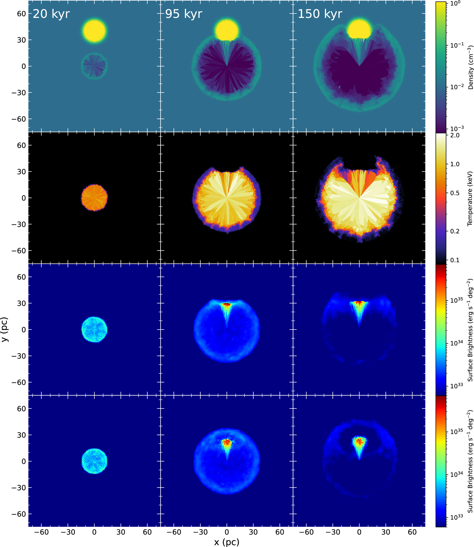
Another potential physical origin of the X-ray shell could be the equatorial wind from the supercritical accretion disk (N. I. Shakura & R. A. Sunyaev 1973; E. M. Churazov et al. 2024), where fast winds have been observed with optical or radio observations (Z. Paragi et al. 1999; I. Waisberg et al. 2019). We estimate the power of the equatorial wind as ∼3 × 1037 erg s−1, based on a mass-loss rate of the gas flow of 10−4 M⊙ yr−1 (I. S. Shkovskii 1981; E. P. J. van den Heuvel 1981; Y. Fuchs et al. 2006) and an average wind terminal velocity of 1000 km s−1 (S. N. Fabrika 1997). This power is optimistically high since the wind velocity drops dramatically to ∼100 km s−1 in areas perpendicular to the jet (S. Fabrika 2004). Nevertheless, the wind power is much smaller than ∼1039 erg s−1, the "average power" of a ∼20 kyr SNR. Based on a self-similar solution of the wind bubble (R. Weaver et al. 1977; M.-M. Mac Low & R. McCray 1988), the plasma would be much cooler (∼0.2 keV) than the fitting result. To further assess this wind scenario, we simulate the evolution of an isotropic wind driven from SS 433 into a uniform diffuse medium with a density of 0.01 cm−3 and also consider a dense cloud at a distance of 40 pc to mimic the dense gas conditions near the Clump. The snapshots of the distribution of density, temperature, and estimated surface brightness at the ages of 20, 95, and 150 kyr are shown in Figure 3. For the estimation of the power of the wind and SN along with the details of the simulation, see Appendix E.

Figure 3. Evolution of a bubble powered by isotropic disk winds with a power of 3 × 1037 erg s−1 within a uniform medium and a dense cloud in the north. From top to bottom, the rows show the evolution of the density, temperature, and X-ray surface brightness in 0.4–2.5 keV. The bottom panels give the surface brightness evolution for the case where the cloud is rotated 41 4 toward us (so that it is projected 30 pc north of SS 433). From left to right, the age of the wind bubble is 20, 95, and 150 kyr, respectively, corresponding to the age of the SNR, the beginning of the collision with the dense cloud, and the later evolution of the wind bubble.
Download figure:
Standard image High-resolution imageOur simulation shows that it would take ∼95 kyr for the winds to blow out a cavity with a radius of the minor axis of W50. The challenge is that the wind is not strong enough for the observed X-ray flux and the gas temperature. The brightest emission appears where the winds interact with the cloud, but the surface brightness is still only half of the observed value of the Clump, especially when projection effects are taken into consideration (see Appendix E for more details). Without a wind–cloud interaction, other parts of the wind bubble are significantly fainter than the region Shell. Besides, we found that the temperature of the wind bubble is inconsistent with the observation. At around 95 kyr, the bubble shell has a temperature of ≲0.5 keV (see Figure 3), significantly cooler than that obtained from the observation. Theoretically, the temperature of the wind shell declines with age due to adiabatical cooling (see Equation (E4)). The shell should thus be hotter at an earlier age, and the simulation gives an effective temperature (emissivity-weighted) of ∼0.6 keV for the shell at 20 kyr. At the wind–cloud interaction region where X-rays are enhanced, the effective temperature is less than 0.6 keV, either in the surface brightness peak (∼90 kyr) or later evolution (150 kyr as an example). Moreover, a longer evolution timescale of the wind compared to the SNR scenario likely suggests a larger ionization timescale so that the plasma could be in or close to the CIE state. Therefore, we conclude that the equatorial disk wind cannot describe the shell-like X-ray emission north of SS 433.
4.2. Progenitor Mass of the Compact Object in SS 433
As shown above, an SNR provides the best explanation for the newly discovered X-ray structure. Our X-ray study and the previously measured black hole mass of 5–15 M⊙ in SS 433 (D. R. Gies et al. 2002; M. G. Bowler 2018; A. M. Cherepashchuk et al. 2019) provide crucial information about the initial stellar mass and the SN properties for creating a black hole. Here we discuss the progenitor mass of the black hole in SS 433 using the pre-SN core mass as predicted by the stellar evolution models (S. E. Woosley & A. Heger 2007, 2015; T. Sukhbold & S. E. Woosley 2014; T. Sukhbold et al. 2016) along with core-collapse SN explosion models (W. Zhang et al. 2008; T. Sukhbold et al. 2016; C. L. Fryer et al. 2018). Figure 4 shows the pre-SN He core masses and the compact remnant mass as a function of the zero-age main-sequence (ZAMS) stellar mass for stars with solar metallicity.

Figure 4. Left panel: mass "budget" of the compact object. The blue solid line represents the mass of the He core (T. Sukhbold et al. 2016). Yellow diamonds and green triangles correspond to models with a given explosion energy (W. Zhang et al. 2008). Gray upper limits label the maximum compact remnant mass among different explosion parameters with a given progenitor mass (C. L. Fryer et al. 2018). The other scatter points are adopted from four different central engines (T. Sukhbold et al. 2016), and only cases with a compact object mass over 2 M⊙ are shown here. Right panel: mass of black holes with successful SN explosion as a function of the explosion energy. Blue stars are given by T. Sukhbold et al. (2016), while orange triangles (20 M⊙) and green diamonds (25 M⊙) are from C. L. Fryer et al. (2018). Only cases where the black hole mass exceeds 2 M⊙ are reserved.
Download figure:
Standard image High-resolution imagePrevious studies suggest that the He core mass sets the upper limit of the compact object mass (W. Zhang et al. 2008; T. Sukhbold et al. 2016). For stars with initial mass ranging from 15 to 30 M⊙, we fitted the data given by T. Sukhbold et al. (2016) and found that there exists an approximate linear relation between stellar initial mass MZAMS and the final mass of He core MHe:

Above ∼40 M⊙, the massive star strips most of the envelope mass with strong stellar winds and ends with an intermediate-mass core. To create a 5 M⊙ compact object, one needs a progenitor star more massive than ∼17 M⊙, while a 10 M⊙ compact object infers the progenitor mass range of ∼30–50 M⊙. Nevertheless, this estimate can be oversimplified, as it does not consider the metal masses taken away by SN ejecta or the explosion parameters that significantly influence the final remnant mass.
Theoretical studies predict a wide diversity of SNe from these very massive stars, from failed SNe (stars that quietly collapse to black holes; C. S. Kochanek 2014) to "hypernovae" with erg (K. Nomoto et al. 2013). To explore the dependence of the compact remnant mass on the explosion energy, we adopt the predicted results from three SN explosion models for stars with solar metallicities (W. Zhang et al. 2008; T. Sukhbold et al. 2016; C. L. Fryer et al. 2018). Two of these models are taken from W. Zhang et al. (2008) for explosion energies of ∼1.2 × 1051 erg and ∼2.4 × 1051 erg. Four models from T. Sukhbold et al. (2016) applied different central engines (N20, K. Nomoto & M. Hashimoto 1988; W15, S. E. Woosley et al. 2002; S19.8, S. E. Woosley et al. 2002; and W18, T. Sukhbold et al. 2016) and provided a range of explosion energies (we only take those producing a remnant mass over 2.5 M⊙ and with SN explosions). We also used models from C. L. Fryer et al. (2018) that calculate the remnant masses and explosion energies for stars with initial masses of 15, 20, and 25 M⊙.

Figure 4(a) illustrates the modeled remnant mass with the ZAMS stellar mass. The remnant masses from the SN models are much smaller than the He-core-confined mass, showing that a substantial amount of material is ejected in the SN explosion. Despite some differences, all these explosion models found that ≳5 M⊙ compact objects are made by stars ≳25 M⊙. As shown in Figure 4(b), explosion energy strongly influences the compact remnant mass, with a heavier remnant favoring a less energetic explosion.
Therefore, the normal SN explosion energy (0.7/1.1 ×1051 erg) for W50 and the 5–15 M⊙ compact object in SS 433 (S. Fabrika 2004; P. T. Goodall et al. 2011; J. S. Farnes et al. 2017) suggests that this binary system contained a progenitor star with a mass ≳25 M⊙. It is noteworthy that the mass of the black hole predicted by SN explosion models does not exceed 8 M⊙, although the upper limit of the black hole mass can be increased for failed SN cases. These models would be challenged if the mass of SS 433 is proven heavier than 8 M⊙. Hence, a more accurate mass measurement of the compact object in SS 433 is of great value.
4.3. Supercritical Accretion Fed by Fallback Disk
The existence of an SNR in W50 provides a stricter constraint on the accretion timescale and an alternative origin of accreted materials. It is thought that supercritical mass transfer of SS 433 occurs due to the accretion from the donor star. To maintain the supercritical accretion, the donor star must be highly evolved and overfill the Roche lobe (S. Fabrika 2004) within 20–30 kyr, the age of the SNR. Because of the short timescale of the post-main-sequence evolution, these two stars in the binary system would share almost the same mass, which happens with a low probability (E. P. J. van den Heuvel 1981).
Alternatively, the accreted material may not purely originate from the companion star, and the SN fallback materials should also be considered. It has already been proposed that some of the young ultraluminous X-ray sources may be black holes accreting from their fallback disks (X.-D. Li 2003), but this hypothesis is waiting for an observational test. Here, we consider that a portion of metal-rich ejecta falls back to SS 433 and provides materials for long-term accretion (X.-D. Li 2003; Q. Han & X.-D. Li 2020), while similar phenomena are observed around some neutron stars but on a smaller scale (e.g., 4U 0142+61, Z. Wang et al. 2006; 1E 161348−5055 in SNR RCW 103, X.-D. Li 2007). On the assumption of a uniform distribution of 1 M⊙ ejecta, we estimate the accretion rate of the fallback disk to be (S. Mineshige et al. 1997; X.-D. Li 2003)

where Mc is the mass of the compact object, Macc is the mass of the fallback materials, α is the viscosity parameter, and t is the age. This is consistent with the observed mass-loss rate of 10−5−10−4 M⊙ yr−1 (I. S. Shkovskii 1981; E. P. J. van den Heuvel 1981; Y. Fuchs et al. 2006). This amount of fallback is possible for creating a black hole (T. Sukhbold et al. 2016; C. L. Fryer et al. 2018), but the exact mass of the fallback materials is still highly uncertain. Further supporting evidence is that the abundance of Ni exceeds the solar value by ∼10 and ∼2, respectively, in the jet and winds of SS 433 (W. Brinkmann et al. 2005; P. S. Medvedev et al. 2018). The Ni enhancement can be naturally explained as nucleosynthesis products released in an SN explosion rather than originating from the donor star's envelope.
4.4. Possible Contributions of an SNR to γ-Ray Emission
W50 has been suggested to be a potential Galactic PeVatron, accelerating particles to hundreds of TeV energies (S. Safi-Harb & R. Petre 1999). After decades of searches for γ-rays from this system, it was finally detected recently in the GeV and high-energy TeV bands (A. U. Abeysekara et al. 2018; K. Fang et al. 2020; J. Li et al. 2020; Z. Cao et al. 2024; H.E.S.S. Collaboration et al. 2024), which has been attributed to the particle acceleration in the jets or winds. The identification of an SNR shell provides us with a new insight into the cosmic-ray acceleration processes occurring in the system. Generally, the γ-ray emission (see Appendix F for details) is extended along the luminous X-ray jet lobes, with the peak emission spatially correlated with nonthermal X-ray knots (A. U. Abeysekara et al. 2018; S. Safi-Harb et al. 2022; H.E.S.S. Collaboration et al. 2024; B. Mac Intyre et al. 2024, in preparation). It is also worth noticing that some portion of the TeV and GeV emission, despite being faint, appears beyond the jet precession cone of SS 433 (K. Fang et al. 2020; J. Li et al. 2020; H.E.S.S. Collaboration et al. 2024). To the west of SS 433, where our study is focused, the TeV γ-ray emission extends to the north in all three bands. The excess seems to have a shell-like morphology, especially above 10 TeV, and shares a similar angular distance to SS 433 with the newly discovered X-ray shell. Unfortunately, the significance of the TeV emission associated with the X-ray shell is ≤2σ based on the current H.E.S.S. data. Modeling of the TeV γ-ray emission suggests a particle acceleration timescale of 1−30 kyr (H.E.S.S. Collaboration et al. 2024), consistent with the SNR age. The interpretation of the recent H.E.S.S. observation suggests that the jets are decelerated to speeds of ∼0.08c by a shock at (30 pc at the distance of 5 kpc) away from SS 433 (H.E.S.S. Collaboration et al. 2024), which would coincide nicely with the location of the X-ray shell. Given that SNRs are in general known to be powerful particle accelerators, it will be crucial to examine the role of the SNR in γ-ray emission in W50 and study the possible interaction between the SNR and jets (S. Safi-Harb et al. 2022).

Acknowledgments
We appreciate the valuable comments and suggestions of the anonymous referee. This study is based on observations obtained with XMM-Newton, an ESA science mission with instruments and contributions directly funded by ESA Member States and NASA. This publication utilizes data from the Galactic ALFA H i (GALFA H i) survey data set obtained with the Arecibo L-band Feed Array (ALFA) on the Arecibo 305 m telescope. The Arecibo Observatory is operated by SRI International under a cooperative agreement with the National Science Foundation (AST-1100968) and in alliance with Ana G. Méndez-Universidad Metropolitana and the Universities Space Research Association. The GALFA H i surveys have been funded by the NSF through grants to Columbia University, the University of Wisconsin, and the University of California. We also acknowledge the use of archival X-ray data downloaded from HEASARC maintained by the NASA Goddard Space Flight Center.
Y.-H.C. acknowledges the foundation from the National Natural Science Foundation of China (NSFC) via grant NSFC 123B1021. The work of P.Z. is supported by grant NSFC 12273010. H.F. acknowledges funding support from the National Natural Science Foundation of China under grant Nos. 12025301, 12103027, and 11821303 and the Strategic Priority Research Program of the Chinese Academy of Sciences. X.-D.L. acknowledges support from the National Key Research and Development Program of China (2021YFA0718500) and the Natural Science Foundation of China under grant Nos. 12041301 and 12121003. S.M. and P.Z. also acknowledge support from Dutch Research Council (NWO) WARP program grant No. 648.003.002, and S.M. acknowledges support from NWO VICI award No. 639.043.513 and European Research Council (ERC) Synergy Grant "BlackHolistic" award No. 101071643. S.S.H. acknowledges the support of the Natural Sciences and Engineering Research Council of Canada (NSERC) through the Canada Research Chairs and Discovery Grants programs and of the Canadian Space Agency.
Software: SAS (C. Gabriel et al. 2004), XSPEC (K. A. Arnaud 1996), Arepo (V. Springel 2010)
Appendix A: ROSAT PSPC Image
Current XMM-Newton data only cover a portion of the nebula W50 and thus fail to give us an overall view. Instead, we applied archival ROSAT (J. Trumper 1982) PSPC data (US400271P, PI: M. Francis; WG500058P; PI: W. Brinkmann; see S. Safi-Harb & H. Ögelman 1997) for reference in favor of its large field of view. We mosaic the PSPC images on a scale of 30'' pixel–1 with the CIAO (A. Fruscione et al. 2006) script reproject_image_grid. To increase the signal-to-noise ratio, we smoothed the PSPC image with a Gaussian kernel with a radius of 3 pixels.
Appendix B: Spectra with Folded Models
Here are the XMM-Newton spectra with folded plasma models. Figure 5(a) gives the spectra of the background. The spectra of the Shell are listed in Figures 5(b), (c), and (d) with the vapec, vnei, and vpshock models, respectively. Figures 5(e) and (f) show the spectra of the Clump with the vapec and vnei models.

Download figure:
Standard image High-resolution image
Figure 5. Spectra with folded models of the regions Shell (left column) and Clump (right column). From top to bottom are the null hypothesis and the vnei, vpshock, vapec, and vapec* models. Different components of the MOS2 spectra are labeled with dashed lines. The null hypothesis spectra mark the astrophysical background from the local hot bubble, galactic halo, and background in yellow, cyan, and blue, respectively. For the others, the astrophysical background is labeled in yellow, while the extra thermal component is marked in cyan. Gray lines represent the Al K fluorescence lines of the instrument background.
Download figure:
Standard image High-resolution imageAppendix C: Significance of Diffuse Emission
Here we quantitatively verify the significance of diffuse emission mainly based on the following two methods. First, the F-test is widely used to tell the significance of an extra component in spectral fittings. 11 It would give a probability based on the chi-square and degrees of freedom of two different models, one of which has an extra component. A smaller probability (e.g., lower than 10−2 or 10−3) indicates higher significance. Besides different models describing the physical property of the diffuse emission mentioned in Section 3, we also test the "null hypothesis" for comparison. Assuming that the diffuse emission originates from the fluctuation, we directly use the background model to fit the source spectra, and the results are also listed in Table 1. Comparing the null hypothesis with the vnei model, the probabilities given by the F-test are 5 × 10⁻³² and 4 × 10⁻¹³ for the Shell and Clump, respectively.
Meanwhile, we study the probability distribution of the emission measure, or rather the parameter norm in Table 1, which is proportional to the unabsorbed flux. As the parameter error is asymmetric and non-Gaussian, we use the XSPEC script steppar to fit the spectra while stepping the value of the emission measure logarithmically from 10−6 to 10−2 cm−5. The chi-square increases rapidly when the emission measure drops below ∼10−5 cm−5 and has a 5σ lower limit around this value as plotted in Figure 6. Therefore, we conclude that the detection of the diffuse emission is robust.

Figure 6. Relation between the change in the chi-square (Δχ2) and the value of the emission measure (in units of cm−5) given by steppar for three models in two regions (blue solid lines). Green dotted lines and orange dashed lines mark the fitting statistics corresponding to the 3σ (Δχ2 = 9) and 5σ (Δχ2 = 25) confidence level. With large degrees of freedom, the chi-square distribution can be approximated as the Gaussian distribution.
Download figure:
Standard image High-resolution imageAppendix D: SNR in the Sedov–Taylor Phase
The physical properties of the Shell are calculated using the fitting results of NEI models. The density depends on the volume of X-ray-emitting gas, and here we assume that the Shell and Clump have an average depth of (approximately the width of the Shell region) at a distance of 5 kpc (Y. Su et al. 2018). The region area is based on the backscal keyword of the spectra. Hence, we estimate the average density of the Shell as


where D ∼ 5 kpc is the distance of W50 (Y. Su et al. 2018). For the Clump where X-ray emission is enhanced, its density is a little higher with .

Noticeably, this density is much lower than that in the X-ray lobe of ∼1 cm−3 95 pc away from SS 433 (W. Brinkmann et al. 2007; S. Safi-Harb et al. 2022), indicative of different gas densities in the two regions. Assuming the X-ray shell is located at the radio boundary of W50 ( to SS 433) but projected inside the nebula, the distance of the Shell to SS 433 is obtained as


and the gas mass swept by the shock Ms (assumed in a uniform medium) is

where mp is the proton mass and n0 = n/4 is the density of preshock gas. As the swept mass exceeds that of the ejecta (in general <10 M⊙; T. Sukhbold et al. 2016), the SNR should have left the free expansion phase and entered the Sedov phase (G. Taylor 1950; L. I. Sedov 1959) when the SNR evolves adiabatically. The shock velocity is also typical for SNRs in the Sedov–Taylor phase but larger than that in the radiative phase (≲200 km s−1; J. Vink 2020).
With the temperature of the plasma, we can derive the shock velocity,

where μ = 0.6 is the mean atomic weight for fully ionized plasma. Assuming a uniform ambient ISM, the age of W50 is

With age in Equation (D5), we can calculate the expected ionization timescale of the hot gas and compare it with the X-ray spectral fitting results,

which is consistent with our spectral analysis (1010−1011 s cm−3). Then we obtained the explosion energy of

where the dimensionless factor ξ = 2.025. This is a typical value for a core-collapse SN (J. Vink 2020).
As a high-mass X-ray binary, SS 433 should have a massive progenitor system, which can drive strong stellar winds to create a large, low-density wind-blown bubble. If the SNR is evolving in a circumstellar medium with a density n ∝ r−2 (r is the distance to the central star), the age is derived as kyr (J. Vink 2020), higher than in a uniform medium but in the same order. In the wind bubble scenario, the dimensionless factor in Equation (D7) can be expressed approximately by J. K. Truelove & C. F. McKee (1999),


where s = 2 for a wind bubble. Applying it along with the age of 28.6 kyr as mentioned above to Equation (D7), the explosion energy would be ∼1.4 × 1051 erg, ∼1.5 times that in a uniform environment. It should be noted that even adopting the fitting results of the CIE model shown in Table 1, the age (Equation (D5)) and explosion energy (Equation (D7)) do not change significantly. Moreover, the expected ionization timescale (Equation (D6)) is still ≲1011 s cm−3, not reaching CIE yet.
Another factor that needs considering is that the heating timescale of electrons can be longer than the age of an SNR (see K. J. Borkowski et al. 2001; P. Ghavamian et al. 2013, and references therein), but in Equation (D4), the electrons and ions are assumed with the same temperature. Here we use the measured ionization timescale τ, although with higher uncertainties compared to the temperature, to recalculate the age in Equation (D5),

and the explosion energy in Equation (D7),

This explosion energy is slightly lower than that given in Equation (D7) but is also reasonable for a core-collapse SNR.
It should be noted that the age and explosion energy here are based on strong assumptions and have uncertainty. Besides the fitting errors in Table 1, the real spatial structure of X-ray-emitting gas is unknown. Meanwhile, the evolution model is based on isotropic explosion and uniform density distribution, while asymmetric explosion may happen for core-collapse SNRs (e.g., L. A. Lopez et al. 2011), and current data reveal the density gradients. Anyhow, the calculation here is still representative, indicating that a black hole could form with a canonical SN.
Appendix E: Equatorial Disk Wind
The equatorial disk wind may also blow out a bubble. For SS 433, the disk wind velocity has been measured based on independent optical and radio observations for the regions with a polar angle α > 60°. The wind velocity is ∼1300 km s−1 and ∼100 km s−1 when α is 60° and 90°, respectively, while an average value is ∼450 km s−1 (S. Fabrika 2004; I. Waisberg et al. 2019). The mass transfer rate as a function of polar angle is unclear, but the total mass-loss rate is 10−4 M⊙ yr−1 (I. S. Shkovskii 1981; E. P. J. van den Heuvel 1981; Y. Fuchs et al. 2006), and it grows as the polar angle α increases (S. Fabrika 2004). For simplicity, we assume the wind is isotropic with a mass-loss rate of M⊙ yr−1 and a wind velocity of vw = 1000 km s−1, which is around the upper limit of the average wind velocity. Assuming a constant wind, the power of the wind is


To compare with the SNR scenario, we also calculate the "average power" of the SN by simply dividing the explosion energy by the age,

which is significantly higher than the power of the equatorial disk wind.
Thus, the disk wind is far from a powerful energy source. For a better illustration, we applied a toy evolution model of a wind bubble based on the self-similar solution (R. Weaver et al. 1977; M.-M. Mac Low & R. McCray 1988). The radius of the bubble R can be expressed as

where L37, t5, and n0 are the wind power, bubble age, and ambient density in units of 1037 erg s−1, 105 yr, and 1 cm−3, respectively. In a wind bubble, the temperature decreases from the center to the edge,

where is the dimensionless distance as the ratio of the distance from the bubble center r to the bubble radius R. Its mean value of the whole bubble is


With this equation and Equation (E3), we can get a relation among the bubble size, temperature, and wind power independent of its age and ambient gas:

Therefore, if the disk wind contributes to the diffuse X-ray emission, the temperature would be significantly lower than the 3σ lower limit (0.71 keV for vnei and 0.55 keV for vpshock) according to spectral analysis of the northern X-ray shell. The index suggests that the temperature is not sensitive to the size of W50 and the wind power.

We use the moving-mesh hydrodynamical software Arepo (V. Springel 2010) to simulate the evolution of the wind-blown bubble and the collision between the isotropic disk wind and a dense cloud 40 pc north of SS 433. The simulation box size is 150 pc × 150 pc × 150 pc. We initially set 5.2 × 10⁵ Voronoi cells, placing a 10 M⊙ black hole particle in the center of the simulation box. The number density of the dense cloud is defined by a spherically symmetric Gaussian distribution. The maximum density is set to 120 cm−3, and its 3σ radial size is , corresponding to a total mass of 25,000 M⊙ given by J. Li et al. (2020). Besides the initial dense cloud, we set a uniform density background of 0.01 cm−3 inferred from our X-ray spectral analysis. The dense cloud and the homogeneous diffuse gas have a uniform initial gas temperature of 104 K.

In every time step of our simulation, we find 32 cells closest to the central black hole and add the corresponding mass, momentum, and kinetic energy of the disk wind to the cells, weighted by the cell solid angles extended to the central point. We include the self-gravity of the gas and multiple cooling mechanisms, which contain thermal bremsstrahlung, hydrogen and helium recombination, and solar-abundance metal line cooling (H. Li et al. 2019). However, we emphasize that neither self-gravity nor cooling play an important role in our simulation.
The simulation is applied until the age of the system reaches 224 kyr. We first let the cloud on the plane perpendicular to the line of sight to better display the number density n and temperature T distributions of the wind bubble in the simulation snapshots. Then, as the X-ray emission looks inside the radio shell (Figure 2), probably due to the projection effect, we also integrate the surface brightness in a direction where the perpendicular distance from the cloud to the central black hole is 30 pc. To estimate the X-ray emission intensity, we use Xspec to calculate the absorbed X-ray emissivity (unit: erg s−1 cm−3) of plasma with a given temperature from 0.1 to 3.0 keV. The foreground column density is set to 7 × 1021 cm2 based on the spectral analysis above. By integrating the emissivity along the line of sight, we can estimate the surface brightness (unit: erg s−1 deg−2) of the bubble in 0.4–2.5 keV. The snapshots of the gas number density, gas temperature, and surface brightness map of our simulation are shown in Figure 3.
Here, we compare the surface brightness (in units of erg s−1 deg−2) between the simulation and observation. We obtained a surface brightness of 1.1 × 1035 erg s−1 deg−2 and 6.1 × 1035 erg s−1 deg−2 for the Shell and the Clump, respectively. During the whole evolution, the surface brightness of the bubble shell is always more than 1 order of magnitude lower than that of the Shell. For the Clump, we select an elliptical region with a major axis of 12 pc and a minor axis of 6 pc (the same size as the region for spectral analysis) and plot the evolution of its average surface brightness in Figure 7(a). This light curve reaches a peak near 90 kyr when the cloud begins to be shocked by the wind. Even the peak surface brightness only reaches half of that of the Clump.

Figure 7. (a) Average surface brightness evolution of the wind bubble in the region Clump. (b), (c), and (d) Normalized luminosity distribution of the temperature in 20, 90, and 150 kyr, respectively. At 20 kyr, the X-ray emission is completely from the shell, as the shock has not arrived at the cloud. At 90 and 150 kyr, the X-rays are dominated by the clump. The last bin (1.6 keV) represents the temperature range above 1.5 keV.
Download figure:
Standard image High-resolution imageThe comparison of the gas temperature is less straightforward since the X-ray emission of our simulation comes from multitemperature plasma, but the spectral analysis is based on a single-temperature model. In Figures 7(b), (c), and (d), we show the normalized X-ray luminosity as a function of the gas temperature for the whole wind-blown bubble at the ages of 20, 90, and 150 kyr. The mean temperature is 0.60, 0.52, and 0.56 keV, respectively, less than that given by the observation. At 20 kyr, the X-ray emission is completely from the shell, as the shock has not arrived at the cloud. At 90 and 150 kyr, the X-rays are dominated by the Clump.
Appendix F: Image of TeV γ-Ray Emission
Here we compare the spatial distribution of X-ray γ-ray emission in different bands in Figure 8. We applied H.E.S.S. (F. Aharonian et al. 2006) data in the TeV band with relatively good spatial resolution (H.E.S.S. Collaboration et al. 2024). To extend the other energy regimes, we also plot associated γ-ray sources detected previously with the Fermi-LAT (W. B. Atwood et al. 2009) data (0.02–300 GeV; J. Li et al. 2020) and LHAASO WCDA (1–25 TeV) and KM2A (>25 TeV) data (Z. Cao et al. 2024).

Figure 8. Spatial relations between X-rays and γ-rays. The dual-band image consists of ROSAT X-ray images of W50 (red) and the significance of H.E.S.S. data in the 0.8–2.5 (a), 2.5–10 (b), and >10 TeV (c) bands (H.E.S.S. Collaboration et al. 2024; cyan). The white contours show the 1.5σ, 3σ, and 4.5σ confidence levels of the TeV emission. The X-ray image is in square-root scale, and the contour levels are 1.5σ, 3.0σ, and 4.5σ. The newly discovered X-ray shell is labeled in green. In the upper panel, the yellow plus signs mark the location of GeV source Fermi J1913+0515 and the "west excess" (J. Li et al. 2020), and the circle stands for the position uncertainty. In the lower panel, the yellow plus signs label LHAASO sources 1LHAASO J1913+0515 (detected by KM2A) and 1LHAASO J1910+0516* (detected by WCDA and KM2A; Z. Cao et al. 2024), with the circles the 1σ extension or 95% extension upper limit of the sources.
Download figure:
Standard image High-resolution image
Footnotes
- 10
- 11
It should be noted that the F-test may be misleading (R. Protassov et al. 2002), but it still has a qualitative meaning here as the detection is evident.