


| Algorithm 1: Compute x and ΛSI |
| Step 1: Solve Ax=e1 by using any symmetric Toeplitz linear solver Step 2: SI and S have the same first column: x=[x1,x2,…,xn]T Step 3: The entries of ΛSI are computed from √nFnΩnx by applying an FFT |
Citation: Jie Xiong, Geng Deng, Xindong Wang. Extension of SABR Libor Market Model to handle negative interest rates[J]. Quantitative Finance and Economics, 2020, 4(1): 148-171. doi: 10.3934/QFE.2020007
| [1] | Natália Bebiano, João da Providência, Wei-Ru Xu . Approximations for the von Neumann and Rényi entropies of graphs with circulant type Laplacians. Electronic Research Archive, 2022, 30(5): 1864-1880. doi: 10.3934/era.2022094 |
| [2] | Jia-Min Luo, Hou-Biao Li, Wei-Bo Wei . Block splitting preconditioner for time-space fractional diffusion equations. Electronic Research Archive, 2022, 30(3): 780-797. doi: 10.3934/era.2022041 |
| [3] | D. Mosić, P. S. Stanimirović, L. A. Kazakovtsev . The m-weak group inverse for rectangular matrices. Electronic Research Archive, 2024, 32(3): 1822-1843. doi: 10.3934/era.2024083 |
| [4] | Ming-Kai Wang, Cheng Wang, Jun-Feng Yin . A class of fourth-order Padé schemes for fractional exotic options pricing model. Electronic Research Archive, 2022, 30(3): 874-897. doi: 10.3934/era.2022046 |
| [5] | Xiu-Jian Wang, Jia-Bao Liu . Quasi-tilted property of generalized lower triangular matrix algebras. Electronic Research Archive, 2025, 33(5): 3065-3073. doi: 10.3934/era.2025134 |
| [6] | Asima Razzaque, Abdul Razaq, Sheikh Muhammad Farooq, Ibtisam Masmali, Muhammad Iftikhar Faraz . An efficient S-box design scheme for image encryption based on the combination of a coset graph and a matrix transformer. Electronic Research Archive, 2023, 31(5): 2708-2732. doi: 10.3934/era.2023137 |
| [7] | Jiachen Mu, Duanzhi Zhang . Multiplicity of symmetric brake orbits of asymptotically linear symmetric reversible Hamiltonian systems. Electronic Research Archive, 2022, 30(7): 2417-2427. doi: 10.3934/era.2022123 |
| [8] | Yang Song, Beiyan Yang, Jimin Wang . Stability analysis and security control of nonlinear singular semi-Markov jump systems. Electronic Research Archive, 2025, 33(1): 1-25. doi: 10.3934/era.2025001 |
| [9] | Ruiping Wen, Liang Zhang, Yalei Pei . A hybrid singular value thresholding algorithm with diagonal-modify for low-rank matrix recovery. Electronic Research Archive, 2024, 32(11): 5926-5942. doi: 10.3934/era.2024274 |
| [10] | Cairong Chen . A structure-preserving doubling algorithm for solving a class of quadratic matrix equation with M-matrix. Electronic Research Archive, 2022, 30(2): 574-584. doi: 10.3934/era.2022030 |
There have been extensive studies and applications of Toeplitz and quasi-Toeplitz matrices recently. Toeplitz or quasi-Toeplitz matrices are adopted as a core tool in the quantum magnetic field [1], generation of random bits [2], quantum key distribution [3,4,5], the evaluation of the short-time rate of change in the trend of CO2 data [6], the deconvolution of hemodynamic responses [7] and the scattering and radiation on thin wire models [8]. Some studies have utilized Toeplitz or quasi-Toeplitz matrices to solve the ordinary and partial differential equations [9,10], also applying them to solve the fractional differential equations [11,12,13,14,15,16].
A large number of linear systems with Toeplitz coefficient matrices need to be solved. Recently, Liu et al. developed fast solvers for Toeplitz linear systems [17,18,19]. The inversion of the Toeplitz matrix is represented as a combination of circulant and skew-circulant matrices in [20,21] so that the solution can be gained directly by using the fast Fourier transform (FFT) and the inverse FFT (IFFT). Here, we turn to express the Toeplitz inversion by using the sum products of the skew-imaginary circulant [22] and skew-circulant matrices, where the skew-imaginary circulant matrix is an ω-circulant matrix with ω=−i, i=√−1.
Regarding the design of fast algorithms for a quasi-Toeplitz linear system, the authors of [23] presented new efficient algorithms to solve the CUPL-Toeplitz linear system [24,25,26] by first splitting the CUPL-Toeplitz matrix into a Toeplitz matrix and a low-rank matrix. In [27], Zhang et al. studied order-reduction algorithms to further reduce the computation complexity. The tridiagonal quasi-Toeplitz linear system is solved in [28].
We are concerned with a class of quasi-symmetric Toeplitz linear systems. The authors of [18] showed the trigonometric transformation splitting method to solve the real symmetric Toeplitz linear system. Different from the iterative method, we adopt the direct method based on the symmetric Toeplitz inversion representation, which is simplified due to the symmetry. We also show the numerical stability of the splitting symmetric Toeplitz inversion inspired by previous studies [26,29,30].
In this paper, we study an n×n real symmetric Toeplitz matrix with perturbations in the first and last columns P=(pj,k)nj,k=1∈Rn×n:
| pj,k={ς1+t1,j=2 and k=1,ς2+t1,j=n−1 and k=n,t|j−k|, otherwise. | (1.1) |
Obviously,
| P=A+αeT1+βeTn, | (1.2) |
where α=[0,ς1,0,…,0]T, e1=[1,0,…,0]T is the first unit vector, β=[0,…,0,ς2,0]T, en=[0,…,0,1]T is the last unit vector and A=(t|j−k|)nj,k=1 is a nonsingular symmetric Toeplitz matrix.
An outline of this paper is as follows. Section 2 solves a sequence of linear systems with the same symmetric Toeplitz coefficient matrix. Section 3 presents the solvers for the quasi-symmetric Toeplitz linear system. A discussion of the quasi-symmetric Toeplitz matrix-vector multiplication is presented in Section 4. In Section 5, the stability analysis of the splitting inverse of the symmetric Toeplitz matrix is shown. Different numerical examples are given in Section 6. In Section 7, images are encrypted and decrypted by using the proposed quasi-symmetric Toeplitz matrix. Finally, we express our conclusions in Section 8.
The starting point of the algorithms derived in this paper is the following inversion formula of Toeplitz matrices:
Lemma 1. [31,p. 738] Let A=(tj−k)nj,k=1∈Rn×n be a Toeplitz matrix. If the vectors x=[x1,x2,…,xn]T, x1≠0 and y=[y1,y2,…,yn])T are the solutions of the linear systems
| Ax=e1andAy=en. | (2.1) |
Then A is invertible and
| A−1=−1x1(i+1)(SI1S1−SI2S2), | (2.2) |
where SI1 and SI2 are skew-imaginary circulant matrices [22] holding the first columns as x=[x1,x2,…,xn]T and ˜y=[iyn,y1,y2,…,yn−1]T respectively; S1 and S2 are skew-circulant matrices with the first columns ˆy=[−yn,y1,y2,…,yn−1]T and x=[x1,x2,…,xn]T respectively.
Note that we are concerned with a symmetric Toeplitz matrix A; then, the special structure means that the solutions x and y in Eq (2.1) satisfy y=Jx, where the matrix J is an anti-identity matrix of order n.
If Ax=e1 has the solution x=[x1,x2,…,xn]T and x1≠0, then the symmetric Toeplitz matrix A is invertible and Eq (2.2) can be rewritten as
| A−1=1x1(i+1)(SIST+iS∗IS), | (2.3) |
where SI and S have the same first column x=[x1,x2,…,xn]T and the symbol S∗I denotes the conjugate transpose of SI.
Performing the diagonalization scheme on the skew-imaginary circulant matrix, that is, SI=Ω∗nF∗nΛSIFnΩn, we can obtain
| A−1=1x1(i+1)Ω∗nF∗n(ΛSIFnΩnST+iΛ∗SIFnΩnS), | (2.4) |
where Fn=(Fj,k)nj,k=1, Fj,k=1√ne2πi(j−1)(k−1)n, 1≤j,k≤n, Ωn=diag(1,e−3iπ2n,…,e−3i(n−1)π2n) and ΛSI is a diagonal matrix containing the eigenvalues of SI.
Equation (2.4) shows a new decomposition of the symmetric Toeplitz inversion. By taking full account of the structural characteristics of the symmetric matrix, we solve only one system Ax=e1 instead of two linear systems.
In the case of solving a sequence of linear systems with the same coefficient matrix, it is effective to solve Ax=e1 first and then use the new decomposition of the inverse of the symmetric Toeplitz matrix for calculation. Therefore, Algorithm 1 is proposed for the computation of x and the eigenvalues of SI. By applying Eq (2.4), an order-reduction algorithm [27] and FFT and IFFT operations, Algorithm 2 realizes the product of A−1 and v in the real number fields.
| Algorithm 1: Compute x and ΛSI |
| Step 1: Solve Ax=e1 by using any symmetric Toeplitz linear solver Step 2: SI and S have the same first column: x=[x1,x2,…,xn]T Step 3: The entries of ΛSI are computed from √nFnΩnx by applying an FFT |
 DownLoad:
CSV
DownLoad:
CSV
| Algorithm 2: An algorithm for z=A−1v in the real number field |
| Step 1: Calculate the vectors vST=STv and vS=Sv by using Algorithm 1 in [27] Step 2: Calculate ˜v=ΛSIFnΩnvST+iΛ∗SIFnΩnvS by applying the FFT Step 3: Calculate z=1x1(i+1)Ω∗nF∗n˜v by applying Eq (2.4) and IFFT |
DownLoad:
CSV
In the proposed algorithms, the diagonal matrix can be represented by a vector containing the diagonal entries; then, the multiplication of the diagonal matrix and the vector is implemented by using a dot product, thus reducing the storage and computational complexity.
To solve a sequence of linear systems with a constant symmetric Toeplitz coefficient matrix, Algorithm 1 only needs to be computed once. The first step in Algorithm 1 is to solve the symmetric Toeplitz linear system Ax=e1. Any symmetric Toeplitz linear solver can be used, such as the generalized minimal residual (GMRES) method, simplified quasi-minimal residual method, conjugate gradient (CG) method, etc. Since A is set as a symmetric positive definite matrix in our numerical experiments in this paper, we choose a the preconditioned CG (PCG) method with the Strang circulant preconditioner [32] to solve it. The workload of Algorithm 1 is considered to be O(nlog2n).
One FFT or IFFT needs 5nlog2n+O(n) real arithmetic operations [33,p. 75], and one run of Algorithm 1 in [27] needs 15n2log2n+O(n). Algorithm 2 mainly consists of two FFTs, one IFFT and two runs of Algorithm 1 in [27]. In the first step of Algorithm 2, it can save two FFTs with the length n2 when calculating STv and Sv simultaneously. Finally, we regard the workload of Algorithm 2 as 25nlog2n+O(n). The application of the order-reduction algorithm reduces the entire computational complexity.
A sequence of Toeplitz linear systems with the same coefficient matrix is solved in [20,21,34]. The method of using the splitting Toeplitz matrix inversion greatly saves the computational time. This reminds us that in a mathematical or engineering problem, we may be faced with thousands of linear systems with the same symmetric Toeplitz matrix. By applying Algorithm 2, it will be more efficient to solve these symmetric Toeplitz linear systems.
In this section, we solve a real quasi-symmetric Toeplitz linear system
| Pa=b, | (3.1) |
where a=[a1,a2,…,an]T is an unknown vector and b=[b1,b2,…,bn]T is known. The coefficient matrix has a decomposition shown in Eq (1.2). We substitute Eq (1.2) into Eq (3.1) and multiply both sides of the equation by A−1 from the left; given that In is an identity matrix, we have
| (In+A−1αeT1+A−1βeTn)a=A−1b. | (3.2) |
Let A−1α=μ, A−1β=ν and A−1b=η, where μ=[μ1,μ2,…,μn]T, ν=[ν1,ν2,…,νn]T and η=[η1,η2,…,ηn]T. The solution of Eq (3.2) can be
| a=(In+μeT1+νeTn)−1η. | (3.3) |
Therefore, solving Pa=b is the same as calculating Eq (3.3). Based on the Sherman-Morrison-Woodbury (SMW) formula [35], (In+μeT1+νeTn)−1 can be represented as
| (In+μeT1+νeTn)−1=In−C, | (3.4) |
where C=(cj,k)nj,k=1 and
| cj,k={(1+νn)μj−μnνj(1+μ1)(1+νn)−μnν1,k=1,(1+μ1)νj−ν1μj(1+μ1)(1+νn)−μnν1,k=n,0,otherwise. | (3.5) |
According to Eqs (3.3)–(3.5), we have
| a=(In−C)η=(ηj−cj,1η1−cj,nηn)nj=1. | (3.6) |
To solve the linear system Pa=b, we must solve the symmetric Toeplitz systems Aμ=α, Aν=β and Aη=b at first. By using Algorithms 1 and 2 and Eqs (3.5) and (3.6), we obtain the following:
| Algorithm 3: An algorithm to solve the real quasi-symmetric Toeplitz system Pa=b |
| Step 1: Run Algorithm 1 Step 2: Calculate μ=A−1α, ν=A−1β and η=A−1b by using Algorithm 2 Step 3: Calculate cj,k by using Eq (3.5) Step 4: Calculate a by using Eq (3.6) |
DownLoad:
CSV
Similarly, if we multiply Eq (1.2) by A−1 from the right, we can get P=(In+αeT1A−1+βeTnA−1)A and substitute it into Eq (3.1); then,
| (In+αeT1A−1+βeTnA−1)Aa=b. | (3.7) |
Denote eT1A−1=ρT, eTnA−1=σT and Aa=ψ, where ρ=[ρ1,ρ2,…,ρn]T, σ=[σ1,σ2,…,σn]T and ψ=[ψ1,ψ2,…,ψn]T. Then, Eq (3.7) can be rewritten as
| ψ=(In+αρT+βσT)−1b. | (3.8) |
The SMW formula is applied to Eq (3.8); we can write
| (In+αρT+βσT)−1=In−D, | (3.9) |
where D=(dj,k)nj,k=1 and
| dj,k={(1+σn−1ς2)ς1ρk−ρn−1ς1ς2σk(1+ρ2ς1)(1+σn−1ς2)−σ2ρn−1ς1ς2,j=2,(1+ρ2ς1)ς2σk−σ2ς1ς2ρk(1+ρ2ς1)(1+σn−1ς2)−σ2ρn−1ς1ς2,j=n−1,0,otherwise. | (3.10) |
From Eqs (3.8)–(3.10), we can get
| ψ=(In−D)b=b−[0,n∑k=1d2,kbk,0,…,0,n∑k=1dn−1,kbk,0]T. | (3.11) |
Since A is a symmetric Toeplitz matrix, if eT1A−1=ρT and eTnA−1=σT, then Aρ=e1 and Aσ=en. According to Eqs (3.10) and (3.11) and the proposed algorithms in Section 2, we propose another algorithm for solving Pa=b.
| Algorithm 4: An algorithm to solve the real quasi-symmetric Toeplitz system Pa=b |
| Step 1: Run Algorithm 1; x equals to ρ because Aρ=e1 Step 2: Calculate σ=A−1en according to Algorithm 2 Step 3: Calculate ψ by using Eqs (3.10) and (3.11) Step 4: Calculate a=A−1ψ according to Algorithm 2 |
DownLoad:
CSV
From the above analysis, it is quite evident that the main work of Algorithms 3 and 4 is solving three symmetric Toeplitz linear systems. Moreover, we can omit one calculation of Aρ=e1 in Algorithm 4.
A greater number of symmetric Toeplitz linear systems will need to be solved if there are more perturbations in the coefficient matrix of the quasi-symmetric Toeplitz linear system. It is therefore meaningful to decompose the inverse of the symmetric Toeplitz matrix, as it will save computational time, especially in the case of high-order systems.
In terms of quasi-symmetric Toeplitz matrix-vector multiplication, the symmetric Toeplitz matrix A can be seen as the sum of the circulant and skew-circulant matrices [36], that is,
| Pv=(A+αeT1+βeTn)v=(C+S+αe1T+βeTn)v, | (4.1) |
where v=(v1,v2,…,vn) is the vector and the circulant matrix C and the skew-circulant matrix S are all symmetric.
The first columns of circulant and skew-circulant matrices need to be computed in the splitting step. Considering the symmetry of n-th order A, the first columns of C and S can be obtained by applying the first n2+1 (n is even) or n+12 (n is odd) elements instead of n elements, which can reduce the computation complexity.
Based on the diagonalization scheme of the circulant matrix, C has the spectral decomposition C=F∗nΔCFn, where Fn=(Fj,k)nj,k=1, Fj,k=1√ne2πi(j−1)(k−1)n, 1≤j,k≤n, and ΔC is a diagonal matrix containing the eigenvalues of C. In [27], an order-reduction algorithm for the multiplication of the real skew-circulant matrix and vector is proposed. So the product of the quasi-symmetric Toeplitz matrix and vector can be expressed as
| Pv=F∗nΔCFnv+Sv+αv1+βvn, | (4.2) |
By applying Eq (4.2), the order-reduction algorithm for real skew-circulant matrix-vector multiplication, the FFT and IFFT operations, we give Algorithm 5 for Pv in the real number field as follows.
| Algorithm 5: An algorithm for Pv based on the order-reduction algorithm in the real number field |
| Step 1: Split the n×n symmetric A into the symmetric C and symmetric S, where ck and sk are the first columns of C and S, respectively Step 2: The entries of ΔC are computed from √nFnck by applying an FFT Step 3: Calculate z1=F∗nΔCFnv by applying an FFT, IFFT Step 4: Calculate z2=Sv by applying Algorithm 1 in [27] Step 5: Calculate Pv=z1+z2+αv1+βvn |
DownLoad:
CSV
Because the complexity of one FFT or IFFT is 5nlog2n+O(n) [33,p. 75], Algorithm 1 in [27] needs 15n2log2n+O(n) real arithmetic operations. The complexity of Algorithm 5 is 45n2log2n+O(n), and it consists of one order-reduction algorithm, two FFTs and one IFFT.
We find that the inverse factorization of the symmetric Toeplitz matrix is critical for the solution of quasi-symmetric Toeplitz linear equations. The following is the error analysis of Eq (2.3) in terms of the 1-norm, ∞-norm and 2-norm, respectively. Assume that ˆx=[ˆx1,ˆx2,…,ˆxn]T is the numerical solution of Ax=e1. If ˆx1≠0, we denote
| ˆA−1=1ˆx1(i+1)(^SIˆST+i^SI∗ˆS) | (5.1) |
as a perturbation of A−1, where the forms of ˆSI and ˆS are the same as those in Eq (2.3) and have corresponding perturbations.
Theorem 1. Let ϵ>0; if x1≠0 and ˆx1≠0, suppose that the relative error of 1x1 is ˆϵ=|1/x1−1/ˆx1||1/x1| and
| ‖ˆx−x‖1‖x‖1≤ϵ; | (5.2) |
we get
| ‖A−1−ˆA−1‖1≤|√2x1|{ϵ+[ϵ+(1+ϵ)ˆϵ](1+ϵ)}‖x‖21 | (5.3) |
and
| ‖A−1−ˆA−1‖1‖A−1‖1≤|√2x1|{ϵ+[ϵ+(1+ϵ)ˆϵ](1+ϵ)}‖x‖1. | (5.4) |
Proof. From the representation of A−1 and ˆA−1 and Eqs (2.3) and (5.1), we can get
| ‖A−1−ˆA−1‖1=‖1x1(i+1)(SIST+iS∗IS)−1ˆx1(i+1)(ˆSIˆST+iˆS∗IˆS)‖1=1√2‖1x1SIST+ix1S∗IS−1ˆx1ˆSIˆST−iˆx1ˆS∗IˆS‖1≤1√2‖(1x1SI)ST−(1ˆx1ˆSI)ˆST‖1+1√2‖S∗I(1x1S)−ˆS∗I(1ˆx1ˆS)‖1. | (5.5) |
On the one hand, we can get
| ‖(1x1SI)ST−(1ˆx1ˆSI)ˆST‖1=‖(1x1SI)ST−(1x1SI)ˆST+(1x1SI)ˆST−(1ˆx1ˆSI)ˆST‖1=‖(1x1SI)(ST−ˆST)+(1x1SI−1ˆx1ˆSI)ˆST‖1≤|1x1|⋅‖SI‖1⋅‖ST−ˆST‖1+‖1x1SI−1ˆx1ˆSI‖1⋅‖ˆST‖1. | (5.6) |
According to the structural characteristics of SI and S and Eq (5.2), we note that
| ‖SI‖1=‖x‖1,·‖ST−ˆST‖1=‖x−ˆx‖1≤ϵ‖x‖1,·‖ˆST‖1=‖ˆx‖1≤(1+ϵ)‖x‖1. | (5.7) |
ˆϵ=|1/x1−1/ˆx1||1/x1| is the relative error; then,
| ‖1x1SI−1ˆx1ˆSI‖1=‖1x1x−1ˆx1ˆx‖1=|1x1|⋅‖x−ˆx+(1−x1ˆx1)ˆx‖1≤|1x1|(‖x−ˆx‖1+ˆϵ‖ˆx‖1)≤|1x1|[ϵ+(1+ϵ)ˆϵ]⋅‖x‖1. | (5.8) |
Combining Eqs (5.6)–(5.8), we thus obtain
| ‖(1x1SI)ST−(1ˆx1ˆSI)ˆST‖1≤|1x1|⋅‖x‖21⋅ϵ+|1x1|[ϵ+(1+ϵ)ˆϵ](1+ϵ)⋅‖x‖21=|1x1|{ϵ+[ϵ+(1+ϵ)ˆϵ](1+ϵ)}‖x‖21. | (5.9) |
Similarly, on the other hand,
| ‖S∗I(1x1S)−ˆS∗I(1ˆx1ˆS)‖1≤|1x1|{ϵ+[ϵ+(1+ϵ)ˆϵ](1+ϵ)}‖x‖21. | (5.10) |
Based on Eqs (5.5), (5.9) and (5.10), we can write
| ‖A−1−ˆA−1‖1≤|√2x1|{ϵ+[ϵ+(1+ϵ)ˆϵ](1+ϵ)}‖x‖21. |
By Ax=e1, it is proven that ‖x‖1≤‖A−1‖1, so
| ‖A−1−ˆA−1‖1‖A−1‖1≤|√2x1|{ϵ+[ϵ+(1+ϵ)ˆϵ](1+ϵ)}‖x‖1. |
Theorem 2. Let ϵ>0; if x1≠0, ˆx1≠0 and
| ‖ˆx−x‖1‖x‖1≤ϵ, | (5.11) |
then
| ‖A−1−ˆA−1‖∞≤|√2x1|{ϵ+[ϵ+(1+ϵ)ˆϵ](1+ϵ)}]‖x‖21 | (5.12) |
and
| ‖A−1−ˆA−1‖∞‖A−1‖∞≤|√2x1|{ϵ+[ϵ+(1+ϵ)ˆϵ](1+ϵ)}‖x‖1, | (5.13) |
where ˆϵ=|1/x1−1/ˆx1||1/x1| is the relative error of 1x1.
Proof. Similar to Theorem 1, this proof is based on the same conditions:
| ‖x‖1≤‖A−1‖∞,‖SI‖∞=‖x‖1,‖ˆST‖∞=‖ˆx‖1≤(1+ϵ)‖x‖1, |
| ‖ST−ˆST‖∞=‖x−ˆx‖1≤ϵ‖x‖1 |
and
| ‖1x1SI−1ˆx1ˆSI‖∞=‖1x1x−1ˆx1ˆx‖1≤|1x1|[ϵ+(1+ϵ)ˆϵ]⋅‖x‖1. |
Theorem 3. Under the assumptions and concepts of the previous two theorems, the upper bound of the 2-norm is said to be
| ‖A−1−ˆA−1‖2≤|√2x1|{ϵ+[ϵ+(1+ϵ)ˆϵ](1+ϵ)}‖x‖21 | (5.14) |
and
| ‖A−1−ˆA−1‖2‖A−1‖2≤|√2nx1|{ϵ+[ϵ+(1+ϵ)ˆϵ](1+ϵ)}‖x‖1. | (5.15) |
Proof. As we all know, ‖A−1−ˆA−1‖22≤‖A−1−ˆA−1‖1⋅‖A−1−ˆA−1‖∞; from Eqs (5.3) and (5.12), we have
| ‖A−1−ˆA−1‖2≤|√2x1|{ϵ+[ϵ+(1+ϵ)ˆϵ](1+ϵ)}‖x‖21. |
Recall that
| ‖x‖1≤√n‖x‖2=√n‖A−1e1‖2≤√n‖A−1‖2‖e1‖2=√n‖A−1‖2. | (5.16) |
From Eqs (5.14) and (5.16), we can get
| ‖A−1−ˆA−1‖2‖A−1‖2≤|√2nx1|{ϵ+[ϵ+(1+ϵ)ˆϵ](1+ϵ)}‖x‖1. |
We show the stability analysis of inverse factorization of the symmetric Toeplitz matrix in this section. The absolute and relative perturbation upper bounds are shown in Eqs (5.3) and (5.4), (5.12) and (5.13), (5.14) and (5.15), as far as Ax=e1 is solvable.
In this section, we give some examples for the comparison of different algorithms. The first two examples present a comparison of different quasi-symmetric Toeplitz linear solvers. Examples 3 and 4 are devoted to the fast algorithm for the quasi-symmetric Toeplitz matrix-vector multiplication.
These experiments were done by using MATLAB (R2022a) on a laptop with the following specifications: 16 GB RAM, AMD Ryzen 7 5800H CPU 3.20 GHz. In the following tables, the calculation time is in seconds, "n" denotes the matrix order and "—" indicates that it is out of MATLAB's memory.
Example 1. An n×n quasi-symmetric Toeplitz linear system Pa=b is considered in this example. According to Eq (1.2), the first column of A is (ti)ni=1=1i, and ς1 and ς2 are random values in the range of (0,1). Assume that aexact=[1,1,...,1]T is the exact solution, so the vector b is b=Paexact.
A comparison of the error and time required to solve a quasi-symmetric Toeplitz linear system is presented in Table 1. The derived two algorithms for solving Pa=b are shown in the table as Algorithms 3 and 4. Based on Algorithm 3, AlgHuang Ⅰ replaces Steps 1 and 2 with Huang's algorithm [20,21] for solving three symmetric Toeplitz systems. Similarly, AlgHuang Ⅱ was executed based on Algorithm 4. The back-slash method means solving Pa=b directly by using the back-slash operator in MATLAB. "Error" was set to be ‖a−aexactaexact‖∞, and the stopping criterion for those algorithms, besides Back-slash, was set to be 1×10⁻⁷.
| n | Back-slash | AlgHuang Ⅰ | Algorithm 3 | AlgHuang Ⅱ | Algorithm 4 | |||||||||
| Error | Time | Error | Time | Error | Time | Error | Time | Error | Time | |||||
| 212 | 1.6531e-13 | 0.3730 | 9.7445e-05 | 0.0055 | 6.0940e-07 | 0.0042 | 7.1225e-05 | 0.0053 | 5.6413e-07 | 0.0042 | ||||
| 213 | 3.6759e-13 | 2.1042 | 6.7327e-06 | 0.0110 | 2.4744e-06 | 0.0077 | 8.6325e-06 | 0.0105 | 1.7807e-06 | 0.0072 | ||||
| 214 | 6.9422e-13 | 14.6981 | 1.0160e-05 | 0.0193 | 4.5065e-06 | 0.0149 | 1.2015e-05 | 0.0187 | 6.9125e-06 | 0.0145 | ||||
| 215 | — | — | 1.7506e-05 | 0.0543 | 9.6450e-06 | 0.0374 | 1.7114e-05 | 0.0526 | 1.3520e-05 | 0.0368 | ||||
| ⋮ | ⋮ | ⋮ | ⋮ | ⋮ | ⋮ | ⋮ | ⋮ | ⋮ | ⋮ | ⋮ | ||||
| 223 | — | — | 3.3928e-04 | 22.3273 | 2.3274e-05 | 17.2194 | 6.6408e-04 | 20.4695 | 2.5144e-05 | 12.1401 | ||||
| 224 | — | — | 5.0053e-04 | 40.9616 | 2.4198e-05 | 30.3279 | 4.4434e-04 | 38.0793 | 3.3228e-05 | 23.7662 | ||||
DownLoad:
CSV
Algorithms 3 and 4 have significate superiority over the other methods. They can solve high-order quasi-symmetric Toeplitz linear systems. However, Back-slash cannot work when the matrix order is above 214. The proposed Algorithms 3 and 4 have the shortest computational time. They perform better than AlgHuang Ⅰ and AlgHuang Ⅱ in high-order linear systems due to the application of the order-reduction algorithm.
Example 2. Consider another quasi-symmetric Toeplitz linear system Pa=b, the first column of A and that ς1 and ς2 in Eq (1.2) are generated from an open interval (0,1). The sum of the elements in the first column was added to the diagonal entries of A to keep A as a diagonally dominant matrix. The exact solution of the system was set to be aexact=[1,1,...,1]T.
Table 2 shows a comparison of different methods for solving Pa=b for Example 2. AlgPGMRES refers to solving the linear system by using the GMRES method with the preconditioner. Since P is a nonsymmetric matrix, the GMRES method can be utilized to solve Pa=b. In order to accelerate the convergence rate, the Strang circulant preconditioner [32] of the symmetric Toeplitz matrix A was established.
| n | Back-slash | AlgPGMRES | Algorithm 3 | Algorithm 4 | |||||||
| Error | Time | Error | Time | Error | Time | Error | Time | ||||
| 212 | 2.2649e-14 | 0.3658 | 2.7463e-07 | 0.0015 | 8.2994e-09 | 0.0051 | 4.2296e-09 | 0.0051 | |||
| 213 | 3.1530e-14 | 2.8237 | 6.8151e-08 | 0.0026 | 1.1341e-09 | 0.0088 | 6.1199e-10 | 0.0083 | |||
| 214 | 4.7296e-14 | 20.7760 | 2.0729e-08 | 0.0043 | 4.9841e-08 | 0.0150 | 9.4785e-08 | 0.0136 | |||
| 215 | — | — | 1.1276e-08 | 0.0091 | 1.2811e-08 | 0.0316 | 1.2697e-08 | 0.0301 | |||
| ⋮ | ⋮ | ⋮ | ⋮ | ⋮ | ⋮ | ⋮ | ⋮ | ⋮ | |||
| 223 | — | — | 1.7832e-08 | 2.7828 | 3.2381e-08 | 12.1427 | 3.8938e-08 | 7.1750 | |||
| 224 | — | — | 7.2746e-09 | 5.9250 | 1.0605e-08 | 24.9603 | 2.4069e-08 | 14.3739 | |||
DownLoad:
CSV
According to theoretical analysis, the complexity of Algorithm 4 is lower than that of Algorithm 3. The results show that Algorithm 3 takes more time than Algorithm 4, which is consistent with the theoretical analysis. AlgPGMRES performs better than the other methods. However, compared with the algorithm for solving symmetric systems, the convergence analysis of the GMRES algorithm is very difficult, and there is no clear conclusion at present.
Example 3. Consider the multiplication of Pv. The vector v is Gaussian distributed. The quasi-symmetric Toeplitz matrix P is decomposed as Eq (1.2), where the first column of A is (ti)ni=1=1i and ς1 and ς2 are random values in the range (0,1).
In Table 3, Pv-direct denotes calculation of the quasi-symmetric Toeplitz matrix-vector multiplication via MATLAB. Pv-splitting refers to splitting P according to Eq (4.1) first, and then utilizing the diagonalization scheme of the circulant matrix and skew-circulant matrix for fast calculation. Algorithm 5 is the proposed quasi-symmetric Toeplitz matrix-vector multiplication. Obviously, Algorithm 5 consumed the least amount of time.
| n | Pv-direct | Pv-splitting | Algorithm 5 |
| 212 | 0.0052 | 5.9079e-04 | 6.0490e-04 |
| 213 | 0.0231 | 9.5132e-04 | 9.3785e-04 |
| 214 | 0.0924 | 0.0020 | 0.0017 |
| 215 | — | 0.0034 | 0.0032 |
| ⋮ | ⋮ | ⋮ | ⋮ |
| 222 | — | 0.5931 | 0.5177 |
| 223 | — | 1.2814 | 1.1760 |
| 224 | — | 2.4970 | 2.2437 |
DownLoad:
CSV
Example 4. Consider the multiplication of Pv, the first column of A, ς1 and ς2 in Eq (1.2), and that the vector v are random values in the range (0,1). The sum of the elements in the first column was added to the diagonal entries of A.
Table 4 shows another example for the quasi-symmetric Toeplitz matrix-vector multiplication. As the matrix order increases, the efficiency of Algorithm 5 becomes increases. Our proposed algorithm is suitable for high-order matrix-vector multiplication. However, the Pv-direct method not only takes the longest time, but it also cannot work when the matrix order is above 214.
| n | Pv-direct | Pv-splitting | Algorithm 5 |
| 212 | 0.0040 | 5.7744e-04 | 5.6916e-04 |
| 213 | 0.0191 | 9.7499e-04 | 9.3755e-04 |
| 214 | 0.0624 | 0.0018 | 0.0017 |
| 215 | — | 0.0034 | 0.0031 |
| ⋮ | ⋮ | ⋮ | ⋮ |
| 222 | — | 0.5712 | 0.5041 |
| 223 | — | 1.2831 | 1.1746 |
| 224 | — | 2.5153 | 2.2225 |
DownLoad:
CSV
In the past decades, image encryption and decryption have been widely researched in the area of information security. The results show that the proposed algorithms can be used to encrypt and decrypt images.
Example 1. Based on Eq (1.2), we consider a quasi-symmetric Toeplitz matrix P, where the entries in the first column of A and ς1 and ς2 are random values in the range (0,1). To keep P as a diagonally dominant matrix, we added a parameter to the diagonal entries of P. Images were encrypted and decrypted by left-multiplying by P2 and P−2, respectively.
Figures 1–3 present the effects of image encryption and decryption. The famous figure "Lenna" is taken as an example. Let the original image matrix be X=[x1,x2,…,x256]; the encrypted image matrix can be obtained by matrix-vector multiplication via Algorithm 5, that is, Y=[y1,y2,…,y256]=P(P[x1,x2,…,x256]). The decrypted image matrix can be computed by ˆX=[ˆx1,ˆx2,…,ˆx256]=P−1(P−1[y1,y2,…,y256]). Algorithm 4 was performed for image decryption because of its lower complexity than Algorithm 3.

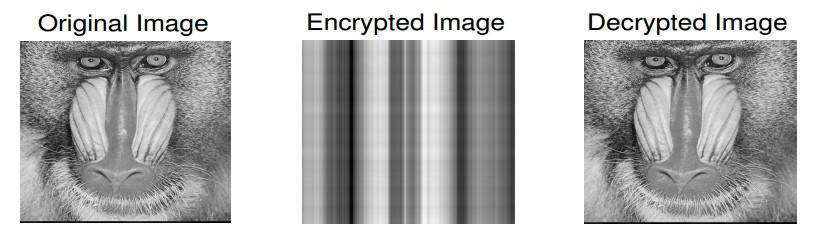
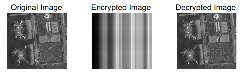
In the process of image encryption and decryption, it is necessary to do multiple matrix-vector multiplications with the same quasi-symmetric Toeplitz matrix and solve linear systems with the same coefficient matrix. Some calculations can be done only once, like Steps 1 and 2 of Algorithm 5 in image encryption, as well as Steps 1 and 2 of Algorithm 4 in image decryption. So, the computational time will be saved.
It is obvious that our proposed algorithms can realize efficient encryption and decryption for different pixel-sized images.
Algorithms for solving a class of real quasi-symmetric Toeplitz linear systems are shown in this paper. We have proposed methods for solving a sequence of linear systems with the constant symmetric Toeplitz matrix based on the decomposition of Toeplitz matrix inversion. By splitting the coefficient matrix into a symmetric Toeplitz matrix plus two low-rank matrices and combining it with the SMW formula, two fast algorithms with O(nlog2n) complexity have been given to solve the real quasi-symmetric Toeplitz linear system. Quasi-symmetric Toeplitz matrix-vector multiplication in the real number field has been presented. Structural perturbation analysis of the inverse factorization of symmetric Toeplitz was also analyzed. Numerical simulations and applications have shown that the proposed algorithms are accurate and efficient.
The research was supported by the National Natural Science Foundation of China (Grant No. 12101284) and Natural Science Foundation of Shandong Province (Grant No. ZR2020MA051).
The authors declare that there is no conflict of interest.
| [1] |
Anderson L, Andreason J (2000) Volatility skews and extensions of the libor market model. Appl Math Financ 7: 1-32. doi: 10.1080/135048600450275

|
| [2] | Antonov A, Konikov M, Spector M (2015) The free boundary SABR: Natural extension to negative rates. Risk. |
| [3] | Balland P, Tran Q (2013) SABR goes normal. Risk, 76-81. |
| [4] |
Brace A (1997) The market model of interest rate dynamics. Math Financ 7: 127-147. doi: 10.1111/1467-9965.00028
|
| [5] | Brigo D, Mercurio F (2006) Interest Rate Models-Theory and Practice, Springer, New York. |
| [6] | Chesney M, Yor M, Jeanblanc M (2009) Mathematical Methods for Financial Markets, Springer, United Kingdom. |
| [7] |
Ferreiro A, García-Rodríguez J, López-Salas J, et al. (2014) SABR/LIBOR market models: Pricing and calibration for some interest rate derivatives. Appl Math Comput 242: 65-89. doi: 10.1016/j.amc.2014.05.017
|
| [8] | Hagan P, Kumar D, Lesniewski A, et al. (2002) Managing smile risk. Wilmott Mag, 84-108. |
| [9] | Henry-Labordere P (2007) Unifying the BGM and SABR models: A short ride in hyperbolic geometry. SSRN. Available from: https://ssrn.com/abstract=877762 or http://dx.doi.org/10.2139/ssrn.877762. |
| [10] |
Honda Y, Inoue J (2019) The effectiveness of the negative interest rate policy in Japan: An early assessment. J Japanese Int Econ 52: 142-153. doi: 10.1016/j.jjie.2019.01.001
|
| [11] |
Joshi M, Rebonato R (2003) A stochastic-volatility displaced-diffusion extension of the LIBOR market model. Quant Financ 3: 458-469. doi: 10.1088/1469-7688/3/6/305
|
| [12] | Kienitz J (2015) Approximate and PDE solution to the boundary free SABR model-application to pricing and calibration. Working Paper. |
| [13] | LeFloch F, Kennedy G (2013) Finite difference techniques for arbitrage free SABR. Working Paper. |
| [14] |
López-Salas J, Vázquez C (2018) PDE formulation of some SABR/LIBOR market models and its numerical solution with a sparse grid combination technique. Comput Math Applications 75: 1616-1634. doi: 10.1016/j.camwa.2017.11.024
|
| [15] | Morini M, Mercurio F (2007) No-arbitrage dynamics for a tractable SABR term structure LIBOR model. Bloomberg Portfolio Res Pap. |
| [16] |
Pedersen H, Swanson N (2019) A survey of dynamic Nelson-Siegel models, diffusion indexes, and big data methods for predicting interest rates. Quant Financ Econ 3: 22-45. doi: 10.3934/QFE.2019.1.22
|
| [17] |
Piterbarg V (2003) A stochastic volatility forward LIBOR model with a term structure of volatility smiles. Appl Math Financ 12: 147-185. doi: 10.1080/1350486042000297225
|
| [18] | Rebonato R (2002) Modern pricing of interest-rate derivatives, Princeton University Press. |
| [19] | Rebonato R (2007) A time-homogeneous, SABR-consistent extension of the LMM: calibration and numerical results. Risk. |
| [20] | Rebonato R, McKay K, White R (2009) The SABR/LIBOR Market Mode: Pricing, Calibration and Hedging for Complex Interest-Rate Derivertives, Wiley, United Kingdom. |
| [21] | Schoenmakers J, Coeffey B (2000) Stable implied calibration of a multi-factor LIBOR model via a semi-parametric correlation structure. WIAS Working Paper. |
| [22] | Wu L, Zhang F (2006) LIBOR market model with stochastic volatility. J Ind Manage Optim 2: 199-227. |
| [23] | Zhu J (2007) An extended LIBOR market model with nested stochastic volatility dynamics. Available at SSRN 955352. |
| 1. | Xin Fan, Ji-Teng Jia, An incomplete tridiagonalization-based determinant evaluation for a generalized periodic tridiagonal matrix, 2024, 1017-1398, 10.1007/s11075-024-01978-7 | |
| 2. | Yi-Fan Wang, Ji-Teng Jia, Xin Fan, A tridiagonalization-based arbitrary-stride reduction approach for (p,q)-pentadiagonal linear systems, 2025, 01689274, 10.1016/j.apnum.2025.02.017 | |
| 3. | Xin Fan, Ji-Teng Jia, Fast breakdown-free algorithm for computing the determinants of a generalized comrade matrix, 2025, 0259-9791, 10.1007/s10910-025-01714-z | |
| 4. | Su-Mei Li, Xin Fan, Yi-Fan Wang, Fast and accurate recursive algorithms for solving cyclic tridiagonal linear systems, 2025, 0259-9791, 10.1007/s10910-025-01716-x |
Figures(16) / Tables(3)

Jie Xiong, Geng Deng, Xindong Wang. Extension of SABR Libor Market Model to handle negative interest rates[J]. Quantitative Finance and Economics, 2020, 4(1): 148-171. doi: 10.3934/QFE.2020007

| Algorithm 1: Compute x and ΛSI |
| Step 1: Solve Ax=e1 by using any symmetric Toeplitz linear solver Step 2: SI and S have the same first column: x=[x1,x2,…,xn]T Step 3: The entries of ΛSI are computed from √nFnΩnx by applying an FFT |
DownLoad:
CSV
| Algorithm 3: An algorithm to solve the real quasi-symmetric Toeplitz system Pa=b |
| Step 1: Run Algorithm 1 Step 2: Calculate μ=A−1α, ν=A−1β and η=A−1b by using Algorithm 2 Step 3: Calculate cj,k by using Eq (3.5) Step 4: Calculate a by using Eq (3.6) |
DownLoad:
CSV
| Algorithm 4: An algorithm to solve the real quasi-symmetric Toeplitz system Pa=b |
| Step 1: Run Algorithm 1; x equals to ρ because Aρ=e1 Step 2: Calculate σ=A−1en according to Algorithm 2 Step 3: Calculate ψ by using Eqs (3.10) and (3.11) Step 4: Calculate a=A−1ψ according to Algorithm 2 |
DownLoad:
CSV
| Algorithm 5: An algorithm for Pv based on the order-reduction algorithm in the real number field |
| Step 1: Split the n×n symmetric A into the symmetric C and symmetric S, where ck and sk are the first columns of C and S, respectively Step 2: The entries of ΔC are computed from √nFnck by applying an FFT Step 3: Calculate z1=F∗nΔCFnv by applying an FFT, IFFT Step 4: Calculate z2=Sv by applying Algorithm 1 in [27] Step 5: Calculate Pv=z1+z2+αv1+βvn |
DownLoad:
CSV
| n | Back-slash | AlgHuang Ⅰ | Algorithm 3 | AlgHuang Ⅱ | Algorithm 4 | |||||||||
| Error | Time | Error | Time | Error | Time | Error | Time | Error | Time | |||||
| 212 | 1.6531e-13 | 0.3730 | 9.7445e-05 | 0.0055 | 6.0940e-07 | 0.0042 | 7.1225e-05 | 0.0053 | 5.6413e-07 | 0.0042 | ||||
| 213 | 3.6759e-13 | 2.1042 | 6.7327e-06 | 0.0110 | 2.4744e-06 | 0.0077 | 8.6325e-06 | 0.0105 | 1.7807e-06 | 0.0072 | ||||
| 214 | 6.9422e-13 | 14.6981 | 1.0160e-05 | 0.0193 | 4.5065e-06 | 0.0149 | 1.2015e-05 | 0.0187 | 6.9125e-06 | 0.0145 | ||||
| 215 | — | — | 1.7506e-05 | 0.0543 | 9.6450e-06 | 0.0374 | 1.7114e-05 | 0.0526 | 1.3520e-05 | 0.0368 | ||||
| ⋮ | ⋮ | ⋮ | ⋮ | ⋮ | ⋮ | ⋮ | ⋮ | ⋮ | ⋮ | ⋮ | ||||
| 223 | — | — | 3.3928e-04 | 22.3273 | 2.3274e-05 | 17.2194 | 6.6408e-04 | 20.4695 | 2.5144e-05 | 12.1401 | ||||
| 224 | — | — | 5.0053e-04 | 40.9616 | 2.4198e-05 | 30.3279 | 4.4434e-04 | 38.0793 | 3.3228e-05 | 23.7662 | ||||
DownLoad:
CSV
| n | Back-slash | AlgPGMRES | Algorithm 3 | Algorithm 4 | |||||||
| Error | Time | Error | Time | Error | Time | Error | Time | ||||
| 212 | 2.2649e-14 | 0.3658 | 2.7463e-07 | 0.0015 | 8.2994e-09 | 0.0051 | 4.2296e-09 | 0.0051 | |||
| 213 | 3.1530e-14 | 2.8237 | 6.8151e-08 | 0.0026 | 1.1341e-09 | 0.0088 | 6.1199e-10 | 0.0083 | |||
| 214 | 4.7296e-14 | 20.7760 | 2.0729e-08 | 0.0043 | 4.9841e-08 | 0.0150 | 9.4785e-08 | 0.0136 | |||
| 215 | — | — | 1.1276e-08 | 0.0091 | 1.2811e-08 | 0.0316 | 1.2697e-08 | 0.0301 | |||
| ⋮ | ⋮ | ⋮ | ⋮ | ⋮ | ⋮ | ⋮ | ⋮ | ⋮ | |||
| 223 | — | — | 1.7832e-08 | 2.7828 | 3.2381e-08 | 12.1427 | 3.8938e-08 | 7.1750 | |||
| 224 | — | — | 7.2746e-09 | 5.9250 | 1.0605e-08 | 24.9603 | 2.4069e-08 | 14.3739 | |||
DownLoad:
CSV
| n | Pv-direct | Pv-splitting | Algorithm 5 |
| 212 | 0.0052 | 5.9079e-04 | 6.0490e-04 |
| 213 | 0.0231 | 9.5132e-04 | 9.3785e-04 |
| 214 | 0.0924 | 0.0020 | 0.0017 |
| 215 | — | 0.0034 | 0.0032 |
| ⋮ | ⋮ | ⋮ | ⋮ |
| 222 | — | 0.5931 | 0.5177 |
| 223 | — | 1.2814 | 1.1760 |
| 224 | — | 2.4970 | 2.2437 |
DownLoad:
CSV
| n | Pv-direct | Pv-splitting | Algorithm 5 |
| 212 | 0.0040 | 5.7744e-04 | 5.6916e-04 |
| 213 | 0.0191 | 9.7499e-04 | 9.3755e-04 |
| 214 | 0.0624 | 0.0018 | 0.0017 |
| 215 | — | 0.0034 | 0.0031 |
| ⋮ | ⋮ | ⋮ | ⋮ |
| 222 | — | 0.5712 | 0.5041 |
| 223 | — | 1.2831 | 1.1746 |
| 224 | — | 2.5153 | 2.2225 |
DownLoad:
CSV
| Algorithm 1: Compute x and ΛSI |
| Step 1: Solve Ax=e1 by using any symmetric Toeplitz linear solver Step 2: SI and S have the same first column: x=[x1,x2,…,xn]T Step 3: The entries of ΛSI are computed from √nFnΩnx by applying an FFT |
| Algorithm 2: An algorithm for z=A−1v in the real number field |
| Step 1: Calculate the vectors vST=STv and vS=Sv by using Algorithm 1 in [27] Step 2: Calculate ˜v=ΛSIFnΩnvST+iΛ∗SIFnΩnvS by applying the FFT Step 3: Calculate z=1x1(i+1)Ω∗nF∗n˜v by applying Eq (2.4) and IFFT |
| Algorithm 3: An algorithm to solve the real quasi-symmetric Toeplitz system Pa=b |
| Step 1: Run Algorithm 1 Step 2: Calculate μ=A−1α, ν=A−1β and η=A−1b by using Algorithm 2 Step 3: Calculate cj,k by using Eq (3.5) Step 4: Calculate a by using Eq (3.6) |
| Algorithm 4: An algorithm to solve the real quasi-symmetric Toeplitz system Pa=b |
| Step 1: Run Algorithm 1; x equals to ρ because Aρ=e1 Step 2: Calculate σ=A−1en according to Algorithm 2 Step 3: Calculate ψ by using Eqs (3.10) and (3.11) Step 4: Calculate a=A−1ψ according to Algorithm 2 |
| Algorithm 5: An algorithm for Pv based on the order-reduction algorithm in the real number field |
| Step 1: Split the n×n symmetric A into the symmetric C and symmetric S, where ck and sk are the first columns of C and S, respectively Step 2: The entries of ΔC are computed from √nFnck by applying an FFT Step 3: Calculate z1=F∗nΔCFnv by applying an FFT, IFFT Step 4: Calculate z2=Sv by applying Algorithm 1 in [27] Step 5: Calculate Pv=z1+z2+αv1+βvn |
| n | Back-slash | AlgHuang Ⅰ | Algorithm 3 | AlgHuang Ⅱ | Algorithm 4 | |||||||||
| Error | Time | Error | Time | Error | Time | Error | Time | Error | Time | |||||
| 212 | 1.6531e-13 | 0.3730 | 9.7445e-05 | 0.0055 | 6.0940e-07 | 0.0042 | 7.1225e-05 | 0.0053 | 5.6413e-07 | 0.0042 | ||||
| 213 | 3.6759e-13 | 2.1042 | 6.7327e-06 | 0.0110 | 2.4744e-06 | 0.0077 | 8.6325e-06 | 0.0105 | 1.7807e-06 | 0.0072 | ||||
| 214 | 6.9422e-13 | 14.6981 | 1.0160e-05 | 0.0193 | 4.5065e-06 | 0.0149 | 1.2015e-05 | 0.0187 | 6.9125e-06 | 0.0145 | ||||
| 215 | — | — | 1.7506e-05 | 0.0543 | 9.6450e-06 | 0.0374 | 1.7114e-05 | 0.0526 | 1.3520e-05 | 0.0368 | ||||
| ⋮ | ⋮ | ⋮ | ⋮ | ⋮ | ⋮ | ⋮ | ⋮ | ⋮ | ⋮ | ⋮ | ||||
| 223 | — | — | 3.3928e-04 | 22.3273 | 2.3274e-05 | 17.2194 | 6.6408e-04 | 20.4695 | 2.5144e-05 | 12.1401 | ||||
| 224 | — | — | 5.0053e-04 | 40.9616 | 2.4198e-05 | 30.3279 | 4.4434e-04 | 38.0793 | 3.3228e-05 | 23.7662 | ||||
| n | Back-slash | AlgPGMRES | Algorithm 3 | Algorithm 4 | |||||||
| Error | Time | Error | Time | Error | Time | Error | Time | ||||
| 212 | 2.2649e-14 | 0.3658 | 2.7463e-07 | 0.0015 | 8.2994e-09 | 0.0051 | 4.2296e-09 | 0.0051 | |||
| 213 | 3.1530e-14 | 2.8237 | 6.8151e-08 | 0.0026 | 1.1341e-09 | 0.0088 | 6.1199e-10 | 0.0083 | |||
| 214 | 4.7296e-14 | 20.7760 | 2.0729e-08 | 0.0043 | 4.9841e-08 | 0.0150 | 9.4785e-08 | 0.0136 | |||
| 215 | — | — | 1.1276e-08 | 0.0091 | 1.2811e-08 | 0.0316 | 1.2697e-08 | 0.0301 | |||
| ⋮ | ⋮ | ⋮ | ⋮ | ⋮ | ⋮ | ⋮ | ⋮ | ⋮ | |||
| 223 | — | — | 1.7832e-08 | 2.7828 | 3.2381e-08 | 12.1427 | 3.8938e-08 | 7.1750 | |||
| 224 | — | — | 7.2746e-09 | 5.9250 | 1.0605e-08 | 24.9603 | 2.4069e-08 | 14.3739 | |||
| n | Pv-direct | Pv-splitting | Algorithm 5 |
| 212 | 0.0052 | 5.9079e-04 | 6.0490e-04 |
| 213 | 0.0231 | 9.5132e-04 | 9.3785e-04 |
| 214 | 0.0924 | 0.0020 | 0.0017 |
| 215 | — | 0.0034 | 0.0032 |
| ⋮ | ⋮ | ⋮ | ⋮ |
| 222 | — | 0.5931 | 0.5177 |
| 223 | — | 1.2814 | 1.1760 |
| 224 | — | 2.4970 | 2.2437 |
| n | Pv-direct | Pv-splitting | Algorithm 5 |
| 212 | 0.0040 | 5.7744e-04 | 5.6916e-04 |
| 213 | 0.0191 | 9.7499e-04 | 9.3755e-04 |
| 214 | 0.0624 | 0.0018 | 0.0017 |
| 215 | — | 0.0034 | 0.0031 |
| ⋮ | ⋮ | ⋮ | ⋮ |
| 222 | — | 0.5712 | 0.5041 |
| 223 | — | 1.2831 | 1.1746 |
| 224 | — | 2.5153 | 2.2225 |
