


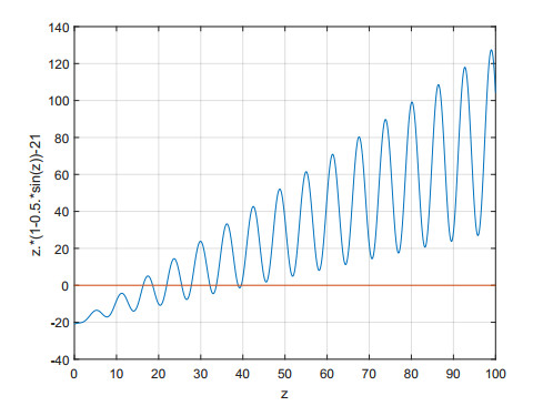
Figure 1.
Nine solutions of 21=z(1−0.5sinz) with z>0 when (a,c,k,k1)=(35,28,0.5,1).
This editorial note is dedicated to the 2023 Journal report of AIMS Materials Science, which was run by AIMS Press. After a brief summary about the annual development in 2023, future developments of the journal in 2024 are proposed. In 2023, AIMS Materials Science received its first Impact Factor (1.8). In addition, based on the Scopus database of Elsevier, the CiteScore of AIMS Materials Science has been increased from 3.3 to 4.2.
Citation: AIMS Materials Science Editorial Office. 2024: Annual Report 2023, AIMS Materials Science, 11(1): 94-101. doi: 10.3934/matersci.2024005
| [1] | Jun Pan, Haijun Wang, Feiyu Hu . Revealing asymmetric homoclinic and heteroclinic orbits. Electronic Research Archive, 2025, 33(3): 1337-1350. doi: 10.3934/era.2025061 |
| [2] | Bin Long, Shanshan Xu . Persistence of the heteroclinic loop under periodic perturbation. Electronic Research Archive, 2023, 31(2): 1089-1105. doi: 10.3934/era.2023054 |
| [3] | Guowei Yu . Heteroclinic orbits between static classes of time periodic Tonelli Lagrangian systems. Electronic Research Archive, 2022, 30(6): 2283-2302. doi: 10.3934/era.2022116 |
| [4] | Xianjun Wang, Huaguang Gu, Bo Lu . Big homoclinic orbit bifurcation underlying post-inhibitory rebound spike and a novel threshold curve of a neuron. Electronic Research Archive, 2021, 29(5): 2987-3015. doi: 10.3934/era.2021023 |
| [5] | Minzhi Wei . Existence of traveling waves in a delayed convecting shallow water fluid model. Electronic Research Archive, 2023, 31(11): 6803-6819. doi: 10.3934/era.2023343 |
| [6] | Anna Gołȩbiewska, Marta Kowalczyk, Sławomir Rybicki, Piotr Stefaniak . Periodic solutions to symmetric Newtonian systems in neighborhoods of orbits of equilibria. Electronic Research Archive, 2022, 30(5): 1691-1707. doi: 10.3934/era.2022085 |
| [7] | Xianjun Wang, Huaguang Gu . Post inhibitory rebound spike related to nearly vertical nullcline for small homoclinic and saddle-node bifurcations. Electronic Research Archive, 2022, 30(2): 459-480. doi: 10.3934/era.2022024 |
| [8] | Xiaochen Mao, Weijie Ding, Xiangyu Zhou, Song Wang, Xingyong Li . Complexity in time-delay networks of multiple interacting neural groups. Electronic Research Archive, 2021, 29(5): 2973-2985. doi: 10.3934/era.2021022 |
| [9] | Peng Mei, Zhan Zhou, Yuming Chen . Homoclinic solutions of discrete p-Laplacian equations containing both advance and retardation. Electronic Research Archive, 2022, 30(6): 2205-2219. doi: 10.3934/era.2022112 |
| [10] | Caiwen Chen, Tianxiu Lu, Ping Gao . Chaotic performance and circuitry implement of piecewise logistic-like mapping. Electronic Research Archive, 2025, 33(1): 102-120. doi: 10.3934/era.2025006 |
This editorial note is dedicated to the 2023 Journal report of AIMS Materials Science, which was run by AIMS Press. After a brief summary about the annual development in 2023, future developments of the journal in 2024 are proposed. In 2023, AIMS Materials Science received its first Impact Factor (1.8). In addition, based on the Scopus database of Elsevier, the CiteScore of AIMS Materials Science has been increased from 3.3 to 4.2.
In this paper, we review a recently reported modified Chen system and examines its singular orbits, giving some new insights into it and extending the existing results [1]. It not only contains the classic Chen system as a special case, but also gives rise to multi-wings attractors with the higher largest Lyapunov exponent. To further understand its nature, we will consider the existence of homoclinic and heteroclinic orbits, which involve some real world applications [2,3,4,5,6,7,8,9], i.e., heart tissue, neurons, cell signalling, chemistry, biomathematics and mechanics, etc. Particularly, when planetary scientists design space missions, the heteroclinic connections between period orbits need to be studied in planar restricted circular three body problem [10,11,12].
For the sake of the following discussion, the concepts of homoclinic and heteroclinic orbits are introduced, i.e., a heteroclinic (resp., homoclinic) orbit is a type of orbit doubly asymptotic to two different equilibrium points or closed orbits (resp., the same equilibrium point or closed orbit) [13,14]. In order to uncover homoclinic and heteroclinic orbits, Shilnikov et al. developed a powerful tool, a combination of contraction map and boundary problem, and categorized chaos of three-dimensional quadratic autonomous differential systems, i.e., chaos of the Shilnikov homoclinic or heteroclinic orbit type, or the hybrid type with both Shilnikov homoclinic and heteroclinic orbits, etc. [14].
With a combination of definitions of the α-limit and ω-limit set and the Lyapunov function, Li et al. revisited the Chen system and proved the existence of a pair of heteroclinic orbits of it [15]. Inspired by that example, other researchers began to consider heteroclinic orbits of other Lorenz-like systems [16,17,18,19,20,21,22,23,24,25] one after another. When studying the Tricomi problem on homoclinic and heteroclinic orbits [26], Leonov formulated the fishing principle and applied it to Lorenz-type systems [27]. Through tracing the stable and unstable manifolds of the Shimizu-Morioka model, Tigan and Turaev [28] detected a pair of homoclinic orbits to the origin. Wiggins, Feng and Hu[13,29] also utilized the Melnikov method to study homoclinic and heteroclinic orbits and, thus, determined chaos in the sense of Smale horseshoes, such as its existence, stability, bifurcation, mutual position between the stable and the unstable manifold, and so on.
More importantly, some bifurcations of homoclinic or heteroclinic orbits may shed light on the problem of the nonlinear relationship between equilibria and the number of multi-wings/scrolls [1,30,31]. Recently, Gilardi-Velázquez et al. [32] collided two heteroclinic orbits to create a new square chaotic attractor, providing a mechanism to establish bistability in a new class of piecewise linear (PWL) dynamical systems. By rupturing heteroclinic-like orbits of a class of PWL systems, Escalante-González and Campos [33] revealed hidden attractors coexisting with self-excited ones.
So far as is known, scholars seldom consider homoclinic and heteroclinic orbits of the modified Chen system [1]. To achieve this target, we reinvestigate it and present the following main contribution:
1) Utilizing a combination of definitions of the α-limit and ω-limit set and the Lyapunov function to prove that there may exist many pairs of heteroclinic orbits to (1) E0 and E± or (2) E+ or (3) E−.
2) Applying a Hamiltonian function to prove that there may exist multitudinous potential homoclinic orbits to E0 and E±, and heteroclinic orbits to E± on the invariant algebraic surface z=x22a.
This paper is organized as follows. The new modified Chen system is introduced and the main results are reported in Section 2. In Section 3, one derives the existence of multitudinous potential homoclinic and heteroclinic orbits. At last, the conclusions are given in Section 4.
In this section, we consider the modified Chen system [1]:
| {˙x=a(y−x),˙y=cy−xz(1−ksin(k1z))+(c−a)x,˙z=−bz+xy, | (2.1) |
where a,c,k,k1,b∈R. Apparently, for k=0, system (2.1) reduces to the Chen system. Of particular interest is that the new added term ksin(k1z) guarantees the creation of multi-wings attractors with higher largest Lyapunov exponent coexisting with multiple equilibria, as illustrated in [1, Figures 2–4, p.2]. Next, we mainly focus on its multiple homoclinic and heteroclinic orbits.
First of all, let us present equilibria of system (2.1):
Proposition 2.1. 1) If b=0, then Ez={(0,0,z)|z∈R} is non-isolated equilibria.
2) When ∀σ≠0, 2c−a=σ[1−ksin(k1σ)], bσ>0, and a≠0. System (2.1) may have many pairs of equilibria: E±={(±√bσ,±√bσ,σ)|bσ>0,2c−a=σ[1−ksin(k1σ)]}, except for E0=(0,0,0).
We arrive at heteroclinic orbits in the case of non-Hamiltonian modified Chen system (2.1):
Proposition 2.2. If 2c>a>c>0, b≥2a>0, ∀σ>0, 2c−a=σ[1−ksin(k1σ)], then
(i) there are no homoclinic orbits to E+ or E−, or heteroclinic orbits to E+ and E− in system (2.1);
(ii) multitudinous potential heteroclinic orbits to (1) E0 and E±, or (2) E+ or (3) E− exist in system (2.1).
Finally, we give homoclinic and heteroclinic orbits on the invariant algebraic surface z=x22a in the following statement.
Proposition 2.3. Suppose c=a, b−2a=0, △=x2−x44a2+2a[akk21sin(k1x22a)−kx22k1cos(k1x22a)], 2a2=x2∗(1−ksin(k1x2∗2a)) and Γ∗=−ax2∗2+x4∗8a−[akk21sin(k1x2∗2a)−kx2∗2k1cos(k1x2∗2a)], then the following two assertions hold.
1) If △≥0, then system (2.1) has a pair of homoclinic orbits to E0: y=x±√△.
2) If △+Γ∗≥0, then system (2.1) has a multitude of heteroclinic or homoclinic orbits to E±: y=x±√△+Γ∗, |x|<|x∗|.
In this section, we first study the existence of heteroclinic orbits when 2c>a>c>0, b≥2a>0, ∀σ>0, and 2c−a=σ[1−ksin(k1σ)], as [15,16,17,18,19,20,21,22,23,24,25].
To facilitate derivation, denote by ϕt(q0)=(x(t;x0),y(t;y0),z(t;z0)) a solution of system (2.1) with the initial value q0=(x0,y0,z0)∈R3. Let γ− (resp., γ+) be the negative (resp., positive) branch of the unstable manifold Wu(E0) corresponding to −x+<0 (resp. x+>0) as t→−∞, i.e., γ∓={ϕ∓t(q0)|ϕ∓t(q0)=(∓x+(t;x0),∓y+(t;y0),z+(t;z0))∈Wu∓(E0),t∈R}.
Put the first Lyapunov function
| V1(ϕt(q0))=V1(x,y,z)=12[2ab(b−2a)σ2c−a(y−x)2+2a(−bz+x2)2+(b−2a)(−bσ+x2)2] |
with the derivative of it along trajectories of system (2.1):
| dV1(ϕt(q0))dt|(2.1)=−2ab(b−2a)σ(a−c)2c−a(y−x)2−2ab(−bz+x2)2 | (3.1) |
for the case of b>2a>0 and sin(k1z)=sin(k1σ), and the second one
| V2(ϕt(q0))=V2(x,y,z)=12[4a2σ(y−x)2+(2c−a)(−2aσ+x2)2] |
with the corresponding derivative:
| dV2(ϕt(q0))dt|(2.1)=−4a2σ(a−c)(y−x)2 | (3.2) |
for the case of b=2a>0, z=x22a and sin(k1x22a)=sin(k1σ).
Here, one only considers the case of heteroclinic orbits to E0 and E±. The other case of heteroclinic orbits to E+ or E− is similar to the ones in [24,25] and is omitted.
For proving Proposition 2.2, one introduces the following result.
Proposition 3.1. When 2c>a>c>0, b≥2a>0, ∀σ>0, and 2c−a=σ[1−ksin(k1σ)], the following two assertions are right.
(i) If ∃ t1,2, such that t1<t2 and V1,2(ϕt1(q0))=V1,2(ϕt2(q0)), then q0 is only one of the equilibria.
(ii) If limϕt(q0)t→−∞=E0, and ∃ t∈R, x(t;x0)<0, then V1,2(E0)>V1,2(ϕt(q0)) and x(t;x0)<0 for all t∈R. Therefore, q0∈Wu−(E0).
Proof. (ⅰ) If 2c>a>c>0, b≥2a>0, ∀σ>0, and 2c−a=σ[1−ksin(k1σ)], then one arrives at dV1,2(ϕt(q0))dt|(2.1)≤0 from Eqs (3.1) and (3.2). On the basis of the hypothesis (ⅰ), one obtains dV1,2(ϕt(q0))dt|(2.1)=0, ∀t∈(t1,t2), and derives that q0 is one stationary point, i.e.,
| ˙x(t;x0)≡˙y(t;y0)≡˙z(t;z0)≡0 | (3.3) |
namely, ˙x(t;x0)=a(y−x)=0 implies x(t)=x0 and ˙y(t,y0)=0, y(t)=y0=0, ∀t∈R.
Since z=x22a is an invariant algebraic surface of system (2.1) with cofactor −2a for b=2a [34], ϕt(q0)∈{y−x=0} results in Eq (3.3).
(ⅱ) Due to limϕt(q0)t→−∞=E0 and x(t;x0)<0, ∃ t∈R, q0 cannot be a fixed point. Otherwise, 0<V1,2(E0)≤V1,2(ϕt0(q0)), ∃t0∈R. Therefore, one arrives at V1,2(ϕt1(q0))≤V1,2(ϕt0(q0)), ∃t1∈R. Based on dV1,2(ϕt(q0))dt|(2.1)≤0, V1,2(ϕt1(q0))=V1,2(ϕt0(q0)) and assertion (ⅰ), q0 is one stationary point. The condition limt→−∞ϕt(q0)=E0 leads to q0=E0 and x(t;x0)=0, ∀t∈R. A contradiction happens. The fact V1,2(E0)>V1,2(ϕt(q0)) holds, ∀t∈R.
Next, let us show x(t,x0)<0, ∀t∈R. If not, ∃ t′∈R, x(t′,x0)≥0. Based on the hypothesis (ⅱ), one obtains x(t″,x0)<0, ∃ t″∈R. As a result, x(τ,x0)=0, ∃ τ∈R. According to V1,2(E0)>V1,2(ϕt(q0)), ∀t∈R, one gets ϕτ(q0)∈{(x,y,z):V1,2(E0)>V1,2(x,y,z)}∩{x=0}, which is contradiction. Actually, both {(x,y,z):V1(E0)>V1(x,y,z)}∩{x=0}={(x,y,z):12[2ab(b−2a)σ2c−ay2+2ab2z2+(b−2a)b2σ2]<(b−2a)b2σ22} and {(x,y,z):V2(E0)>V2(x,y,z)}∩{x=0}={(x,y,z):2a2σy2+2(2c−a)a2σ2<2(2c−a)a2σ2} are all empty. So, ∀t∈R, x(t,q0)<0. The proof is completed.
From Proposition 3.1, one proves Proposition 2.2 as follows.
Proof of Proposition 2.2:. (ⅰ) When 2c>a>c>0, b≥2a>0, ∀σ>0, and 2c−a=σ[1−ksin(k1σ)], there are neither homoclinic orbits to E+ or E−, nor heteroclinic orbits to E+ and E− in system (2.1). Otherwise, suppose p(t)=(x,y,z) is a homoclinic orbit to E′+ or E′−, or heteroclinic orbit to E′±, where ∀E′+∈E+ and ∀E′−∈E−, i.e., limt→−∞p(t)=e−,limt→+∞p(t)=e+, where e− and e+ satisfy either e−=e+∈{E′−,E0,E′+} or {e−,e+}={E′−,E′+}.
Based on dV1,2(ϕt(q0))dt|(2.1)≤0, one arrives at
| V1,2(e−)≥V1,2(p(t))≥V1,2(e+). | (3.4) |
In any case, the relation V1,2(e−)=V1,2(e+) all hold, which also leads to V1,2(p(t))≡V1,2(e−). According to the assertion (ⅰ) of Proposition 3.1, p(t) is just one stationary point. In a word, homoclinic orbits to E+ or E−, or heteroclinic orbits to E+ and E− do not exist in system (2.1).
(ⅱ) Next, one proves that p(t) is a heteroclinic orbit to E0 and E′−, i.e., limt→+∞p(t)=E′−. On the basis of the definition of p(t) and the second assertion of Proposition 3.1, V1,2(E0)>V1,2(p(t)) holds, which also yields limt→+∞p(t)≠E0, i.e., limt→+∞p(t)=E′−.
At last, let us show that, if system (2.1) has a heteroclinic orbit to E0 and E′−, then this orbit is just p(t).
Suppose p∗−(t)=(x∗(t),y∗(t),z∗(t)) is a solution of system (2.1) such that
| limt→−∞p∗−(t)=e−1,limt→+∞p∗−(t)=e+1, |
where e−1 and e+1 satisfy {e−1,e+1}={E0,E′−}. Since dV1,2(ϕt(q0))dt|(2.1)≤0, ∀t∈R, V1,2(e−1)≥V1,2(p∗−(t))≥V1,2(e+1) holds. Due to V1,2(E0)>V1,2(E′−), one gets e−1=E0 and e+1=E′−, i.e.,
| limt→−∞p∗−(t)=E0,limt→+∞p∗−(t)=E′−, |
which yields p∗−(t)∈γ− based on the assertion (ⅱ) of Proposition 3.1. Since system (2.1) is symmetrical w.r.t. the z–axis, there exists a unique heteroclinic orbit p∗+(t)∈γ+, i.e., limt→−∞p∗+(t)=E0,limt→+∞p∗+(t)=E′+.
Due to the term of ksin(k1z), E± may include many isolated stationary points E′± and, thus, may generate many heteroclinic orbits to E0 and E±. The proof is over.
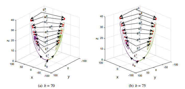
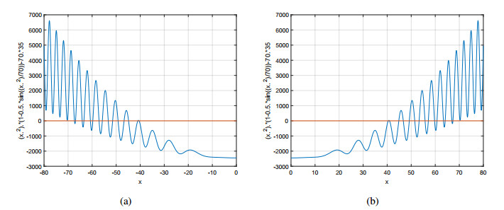
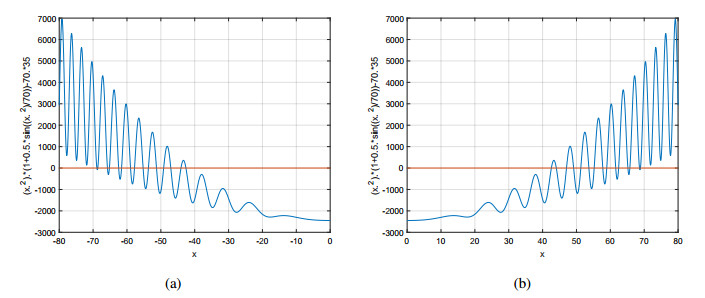
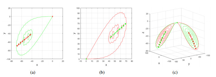
Set (a,c,k,k1)=(35,28,0.5,1), b=70,75. The nontrivial equilibria of system (2.1) satisfies 2c−a=z(1−ksin(k1z)), i.e., 21=z(1−0.5sin(z)) with z>0. At this time, system (2.1) has nine pairs of nontrivial equilibria: Ei±=(±√bzi,±√bzi,zi), where z1=16.319, z2=18.5869, z3=21.9081, z4=25.493, z5=27.7653, z6=32.1844, z7=33.7036, z8=38.8655, and z9=39.6184, as depicted in Figure 1 and Tables 1 and 2.
| E± | Classification | Eigenvalues |
| E1±=(±33.7984,±33.7984,16.319) | Stable focus | −3.5±95.3515i,−70 |
| E2±=(±36.0705,±36.0705,18.5869) | Saddle | 97.589,−104.589,−70 |
| E3±=(±39.1608,±39.1608,21.9081) | Stable focus | −3.5±134.9i,−70 |
| E4±=(±42.2435,±42.2435,25.493) | Saddle | 137.312,−144.312,−70 |
| E5±=(±44.086,±44.086,27.7653) | Stable focus | −3.5±158.18i,−70 |
| E6±=(±47.4648,±47.4648,32.1844) | Saddle | 153.3704,−160.3704,−70 |
| E7±=(±48.5721,±48.5721,33.7036) | Stable focus | −3.5±166.07i,−70 |
| E8±=(±52.1592,±52.1592,38.8655) | Saddle | 135.592,−142.592,−70 |
| E9±=(±52.662,±52.662,39.6184) | Stable focus | −3.5±142.18i,−70 |
 DownLoad:
CSV
DownLoad:
CSV
| E± | Classification | Eigenvalues |
| E1±=(±34.9846,±34.9846,16.319) | Stable focus | −3.5±98.7041i,−75 |
| E2±=(±37.3365,±37.3365,18.5869) | Saddle | 101.1325,−108.1325,−75 |
| E3±=(±40.5353,±40.5353,21.9081) | Stable focus | −3.5±139.64i,−75 |
| E4±=(±43.7261,±43.7261,25.493) | Saddle | 142.2534,−149.2534,−75 |
| E5±=(±45.6333,±45.6333,27.7653) | Stable focus | −3.5±163.73i,−75 |
| E6±=(±49.1307,±49.1307,32.1844) | Saddle | 158.8772,−165.8772,−75 |
| E7±=(±50.2769,±50.2769,33.7036) | Stable focus | −3.5±171.9i,−75 |
| E8±=(±53.9899,±53.9899,38.8655) | Saddle | 140.4712,−147.4712,−75 |
| E9±=(±54.5104,±54.5104,39.6184) | Stable focus | −3.5±147.19i,−75 |
DownLoad:
CSV
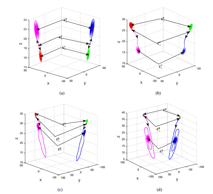
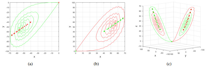
In contrast to the Lorenz-like systems [19,20,24,25], Figures 2–4 show multitudinous heteroclinic orbits to (1) E0 and E±, (2) E+, (3) E−.
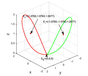
Remark 1. Motivated by [16], a pair of homoclinic orbits to E0 may exist in the scenario of non-Hamiltonian modified Chen system (2.1) when (a,c,k,k1,b)=(1,0.8,0.5,1,1.088966), as shown in Figure 5.
Remark 2. When a=c, V2 is a first integral. Proposition 2.2 includes the result on heteroclinic orbits given in [15,16] as a special case when k=0.
Finally, for b=2a, let us consider homoclinic and heteroclinic orbits on the invariant algebraic surface z=x22a [34] of system (2.1), i.e., the ones of following system:
| {˙x=a(y−x),˙y=cy−x32a[1−ksin(k1x22a)]+(c−a)x. | (3.5) |
When c=a, system (3.5) reduces into a Hamiltonian system with the corresponding Hamiltonian function
| H(x,y)=−axy+a2y2+x48a−[akk21sin(k1x22a)−kx22k1cos(k1x22a)]. | (3.6) |
Obviously, the equilibrium points of system (3.5) are S0=(0,0), S±=(±x,±x) for 2a2=x2(1−ksin(k1x22a)). Further, the proof of Proposition 2.3 easily follows and is omitted here.
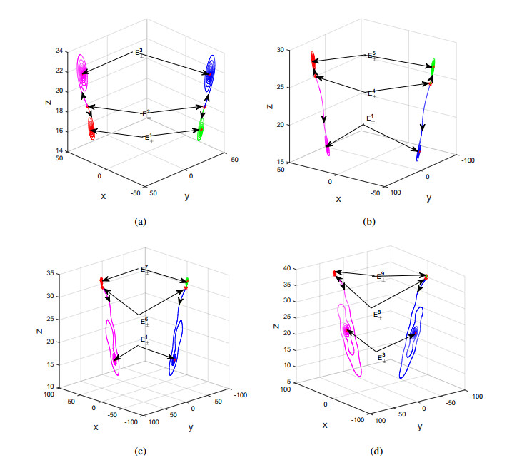
Set (a,c,k,k1)=(±35,±35,0.5,1), except for S0, Figures 6 and 8 show another fifteen pairs of nontrivial equilibria Si± of system (3.5), i.e., the Ei± of system (2.1), i=1,2,⋯,15, as shown in Tables 3 and 4. Obviously, Si± are included in Ei± and are not listed here, i=1,2,⋯,15. Further, system (3.5) (resp., (2.1)) has eight pairs of homoclinic orbits to Si± and S0 (resp., Ei± and E0), i=2,4,6,8,10,12,14, as depicted in Figures 7 and 9. Being different from the ones [25,35], the heteroclinic orbits to Si± (resp., Ei±) are not observed in numerical simulation.
| E± | Classification | Eigenvalues |
| E1±=(±40.4862,±40.4862,23.4162) | Andronov-Hopf bifurcation | ±72.37i,−70 |
| E2±=(±40.9545,±40.9545,23.9610) | Saddle | ±73.1982,−70 |
| E3±=(±44.8424,±44.8424,28.7263) | Andronov-Hopf bifurcation | ±168.62i,−70 |
| E4±=(±46.7089,±46.7089,31.1674) | Saddle | ±174.6572,−70 |
| E5±=(±49.2008,±49.2008,34.5817) | Andronov-Hopf bifurcation | ±210.46i,−70 |
| E6±=(±51.4735, ±51.4735,37.8503) | Saddle | ±217.0728,−70 |
| E7±=(±53.286,±53.286,40.5628) | Andronov-Hopf bifurcation | ±240.47i,−70 |
| E8±=(±55.7622,±55.7622,44.4203) | Saddle | ±245.134,−70 |
| E9±=(±57.1156,±57.1156,46.6027) | Andronov-Hopf bifurcation | ±261.48i,−70 |
| E10±=(±59.7153,±59.7153,50.9417) | Saddle | ±261.5179,−70 |
| E11±=(±60.7207,±60.7207,52.6715) | Andronov-Hopf bifurcation | ±272.84i,−70 |
| E12±=(±63.4129,±63.4129,57.4457) | Saddle | ±263.8527,−70 |
| E13±=(±64.1281,±64.1281,58.7488) | Andronov-Hopf bifurcation | ±271.2i,−70 |
| E14±=(±66.9144,±66.9144,63.9648) | Saddle | ±241.3816,−70 |
| E15±=(±67.3528,±67.3528,64.8057) | Andronov-Hopf bifurcation | ±245.16i,−70 |
DownLoad:
CSV
| E± | Classification | Eigenvalues |
| E1±=(±42.5879,±42.5879,−25.9104) | Shilnikov-Hopf bifurcation | ±138.54i,70 |
| E2±=(±44.0511,±44.0511,−27.7214) | Saddle | ±142.9652,70 |
| E3±=(±47.0547,±47.0547,−31.6306) | Shilnikov-Hopf bifurcation | ±191.48i,70 |
| E4±=(±49.1642,±49.1642,−34.5303) | Saddle | ±198.1574,70 |
| E5±=(±51.2773,±51.2773,−37.5623) | Shilnikov-Hopf bifurcation | ±226.65i,70 |
| E6±=(±53.6664,±53.6664,−41.144) | Saddle | ±232.5816,70 |
| E7±=(±55.2308,±55.2308,−43.5777) | Shilnikov-Hopf bifurcation | ±252.09i,70 |
| E8±=(±57.7749,±57.7749,−47.6848) | Saddle | ±254.8295,70 |
| E9±=(±58.9443,±58.9443,−49.6347) | Shilnikov-Hopf bifurcation | ±268.49i,70 |
| E10±=(±61.5922,±61.5922,−54.1943) | Saddle | ±264.7765,70 |
| E11±=(±62.4478,±62.4478,−55.7104) | Shilnikov-Hopf bifurcation | ±2.7403i,70 |
| E12±=(±65.1845,±65.1845,−60.7003) | Saddle | ±257.1704,70 |
| E13±=(±65.7631,±65.7631,−61.7826) | Shilnikov-Hopf bifurcation | ±262.71i,70 |
| E14±=(±68.6152,±68.6152,−67.2578) | Saddle | ±205.6317,70 |
| E15±=(±68.8911,±68.8911,−67.7998) | Shilnikov-Hopf bifurcation | ±207.64i,70 |
DownLoad:
CSV
In the present work, the existence of homoclinic orbits and heteroclinic orbits of both cases of non-Hamiltonian and Hamiltonian modified Chen system was proved based on definitions of both α-limit set and ω-limit set, the theory of the Lyapunov function, and the Hamiltonian function. In the former case, there existed multitudinous potential heteroclinic orbits to (1) E0 and E±, (2) E+, or (3) E− in that modified Chen system. In the latter case, there was a multitude of potential homoclinic orbits to E0 and E± or heteroclinic orbits to E± on the invariant algebraic surface z=x22a. Moreover, when (a,c,k,k1)=(35,28,0.5,1), b=70,75 (resp., (a,c,k,k1,b)=(±35,±35,0.5,1,±70)), numerical simulations illustrated nine pairs of heteroclinic orbits (resp., eight pairs of homoclinic orbits). What follows is to study the multi-wing Lü system [1], Lorenz system, and other hyperchaotic Lorenz-like systems.
The authors declare they have not used Artificial Intelligence (AI) tools in the creation of this article.
This work is supported in part by the National Natural Science Foundation of China under Grant 12001489, the Zhejiang Public Welfare Technology Application Research Project of China under Grant LGN21F020003, the Natural Science Foundation of Zhejiang Guangsha Vocational and Technical University of Construction under Grant 2022KYQD-KGY, and the Natural Science Foundation of Taizhou University under Grant T20210906033. Meanwhile, the authors would like to express their sincere thanks to the anonymous editors and reviewers for their conscientious reading and numerous constructive comments, which improved the manuscript substantially.
The authors declare there is no conflicts of interest.
| 1. | Feng Ding, Ling Xu, Xiao Zhang, Yihong Zhou, Xiaoli Luan, Recursive identification methods for general stochastic systems with colored noises by using the hierarchical identification principle and the filtering identification idea, 2024, 57, 13675788, 100942, 10.1016/j.arcontrol.2024.100942 | |
| 2. | Guiyao Ke, Jun Pan, Feiyu Hu, Haijun Wang, Dynamics of a New Four-Thirds-Degree Sub-Quadratic Lorenz-like System, 2024, 13, 2075-1680, 625, 10.3390/axioms13090625 | |
| 3. | Ling Xu, Huan Xu, Feng Ding, Adaptive Multi-Innovation Gradient Identification Algorithms for a Controlled Autoregressive Autoregressive Moving Average Model, 2024, 43, 0278-081X, 3718, 10.1007/s00034-024-02627-z | |
| 4. | Siyu Liu, Yanjiao Wang, Feng Ding, Ahmed Alsaedi, Tasawar Hayat, Joint iterative state and parameter estimation for bilinear systems with autoregressive noises via the data filtering, 2024, 147, 00190578, 337, 10.1016/j.isatra.2024.01.035 | |
| 5. | Haijun Wang, Jun Pan, Guiyao Ke, Feiyu Hu, A pair of centro-symmetric heteroclinic orbits coined, 2024, 2024, 2731-4235, 10.1186/s13662-024-03809-4 | |
| 6. | Lijuan Liu, Decomposition‐based maximum likelihood gradient iterative algorithm for multivariate systems with colored noise, 2024, 34, 1049-8923, 7265, 10.1002/rnc.7344 | |
| 7. | Jiayun Zheng, Feng Ding, A filtering‐based recursive extended least squares algorithm and its convergence for finite impulse response moving average systems, 2024, 34, 1049-8923, 6063, 10.1002/rnc.7307 | |
| 8. | Huanqi Sun, Weili Xiong, Feng Ding, Erfu Yang, Hierarchical estimation methods based on the penalty term for controlled autoregressive systems with colored noises, 2024, 34, 1049-8923, 6804, 10.1002/rnc.7323 | |
| 9. | Haoming Xing, Feng Ding, Xiao Zhang, Xiaoli Luan, Erfu Yang, Highly-efficient filtered hierarchical identification algorithms for multiple-input multiple-output systems with colored noises, 2024, 186, 01676911, 105762, 10.1016/j.sysconle.2024.105762 | |
| 10. | Yanjiao Wang, Yiting Liu, Jiehao Chen, Shihua Tang, Muqing Deng, Online identification of Hammerstein systems with B‐spline networks, 2024, 38, 0890-6327, 2074, 10.1002/acs.3792 | |
| 11. | Guiyao Ke, Creation of Three‐Scroll Hidden Conservative Lorenz‐Like Chaotic Flows, 2024, 7, 2513-0390, 10.1002/adts.202400247 | |
| 12. | Haijun Wang, Jun Pan, Guiyao Ke, Revealing More Hidden Attractors from a New Sub-Quadratic Lorenz-Like System of Degree 6 5, 2024, 34, 0218-1274, 10.1142/S0218127424500718 | |
| 13. | Ling Xu, Feng Ding, Xiao Zhang, Quanmin Zhu, Novel parameter estimation method for the systems with colored noises by using the filtering identification idea, 2024, 186, 01676911, 105774, 10.1016/j.sysconle.2024.105774 | |
| 14. | Saida Bedoui, Kamel Abderrahim, Feng Ding, Iterative parameter identification for Hammerstein systems with ARMA noises by using the filtering identification idea, 2024, 38, 0890-6327, 3134, 10.1002/acs.3865 | |
| 15. | Jun Pan, Haijun Wang, Feiyu Hu, Revealing asymmetric homoclinic and heteroclinic orbits, 2025, 33, 2688-1594, 1337, 10.3934/era.2025061 | |
| 16. | Haijun Wang, Jun Pan, Feiyu Hu, Guiyao Ke, Asymmetric Singularly Degenerate Heteroclinic Cycles, 2025, 35, 0218-1274, 10.1142/S0218127425500725 | |
| 17. | Jun Pan, Haijun Wang, Guiyao Ke, Feiyu Hu, Creation of single-wing Lorenz-like attractors via a ten-ninths-degree term, 2025, 23, 2391-5471, 10.1515/phys-2025-0165 |


Figures(6) / Tables(4)

AIMS Materials Science Editorial Office. 2024: Annual Report 2023, AIMS Materials Science, 11(1): 94-101. doi: 10.3934/matersci.2024005

| E± | Classification | Eigenvalues |
| E1±=(±33.7984,±33.7984,16.319) | Stable focus | −3.5±95.3515i,−70 |
| E2±=(±36.0705,±36.0705,18.5869) | Saddle | 97.589,−104.589,−70 |
| E3±=(±39.1608,±39.1608,21.9081) | Stable focus | −3.5±134.9i,−70 |
| E4±=(±42.2435,±42.2435,25.493) | Saddle | 137.312,−144.312,−70 |
| E5±=(±44.086,±44.086,27.7653) | Stable focus | −3.5±158.18i,−70 |
| E6±=(±47.4648,±47.4648,32.1844) | Saddle | 153.3704,−160.3704,−70 |
| E7±=(±48.5721,±48.5721,33.7036) | Stable focus | −3.5±166.07i,−70 |
| E8±=(±52.1592,±52.1592,38.8655) | Saddle | 135.592,−142.592,−70 |
| E9±=(±52.662,±52.662,39.6184) | Stable focus | −3.5±142.18i,−70 |
DownLoad:
CSV
| E± | Classification | Eigenvalues |
| E1±=(±34.9846,±34.9846,16.319) | Stable focus | −3.5±98.7041i,−75 |
| E2±=(±37.3365,±37.3365,18.5869) | Saddle | 101.1325,−108.1325,−75 |
| E3±=(±40.5353,±40.5353,21.9081) | Stable focus | −3.5±139.64i,−75 |
| E4±=(±43.7261,±43.7261,25.493) | Saddle | 142.2534,−149.2534,−75 |
| E5±=(±45.6333,±45.6333,27.7653) | Stable focus | −3.5±163.73i,−75 |
| E6±=(±49.1307,±49.1307,32.1844) | Saddle | 158.8772,−165.8772,−75 |
| E7±=(±50.2769,±50.2769,33.7036) | Stable focus | −3.5±171.9i,−75 |
| E8±=(±53.9899,±53.9899,38.8655) | Saddle | 140.4712,−147.4712,−75 |
| E9±=(±54.5104,±54.5104,39.6184) | Stable focus | −3.5±147.19i,−75 |
DownLoad:
CSV
| E± | Classification | Eigenvalues |
| E1±=(±40.4862,±40.4862,23.4162) | Andronov-Hopf bifurcation | ±72.37i,−70 |
| E2±=(±40.9545,±40.9545,23.9610) | Saddle | ±73.1982,−70 |
| E3±=(±44.8424,±44.8424,28.7263) | Andronov-Hopf bifurcation | ±168.62i,−70 |
| E4±=(±46.7089,±46.7089,31.1674) | Saddle | ±174.6572,−70 |
| E5±=(±49.2008,±49.2008,34.5817) | Andronov-Hopf bifurcation | ±210.46i,−70 |
| E6±=(±51.4735, ±51.4735,37.8503) | Saddle | ±217.0728,−70 |
| E7±=(±53.286,±53.286,40.5628) | Andronov-Hopf bifurcation | ±240.47i,−70 |
| E8±=(±55.7622,±55.7622,44.4203) | Saddle | ±245.134,−70 |
| E9±=(±57.1156,±57.1156,46.6027) | Andronov-Hopf bifurcation | ±261.48i,−70 |
| E10±=(±59.7153,±59.7153,50.9417) | Saddle | ±261.5179,−70 |
| E11±=(±60.7207,±60.7207,52.6715) | Andronov-Hopf bifurcation | ±272.84i,−70 |
| E12±=(±63.4129,±63.4129,57.4457) | Saddle | ±263.8527,−70 |
| E13±=(±64.1281,±64.1281,58.7488) | Andronov-Hopf bifurcation | ±271.2i,−70 |
| E14±=(±66.9144,±66.9144,63.9648) | Saddle | ±241.3816,−70 |
| E15±=(±67.3528,±67.3528,64.8057) | Andronov-Hopf bifurcation | ±245.16i,−70 |
DownLoad:
CSV
| E± | Classification | Eigenvalues |
| E1±=(±42.5879,±42.5879,−25.9104) | Shilnikov-Hopf bifurcation | ±138.54i,70 |
| E2±=(±44.0511,±44.0511,−27.7214) | Saddle | ±142.9652,70 |
| E3±=(±47.0547,±47.0547,−31.6306) | Shilnikov-Hopf bifurcation | ±191.48i,70 |
| E4±=(±49.1642,±49.1642,−34.5303) | Saddle | ±198.1574,70 |
| E5±=(±51.2773,±51.2773,−37.5623) | Shilnikov-Hopf bifurcation | ±226.65i,70 |
| E6±=(±53.6664,±53.6664,−41.144) | Saddle | ±232.5816,70 |
| E7±=(±55.2308,±55.2308,−43.5777) | Shilnikov-Hopf bifurcation | ±252.09i,70 |
| E8±=(±57.7749,±57.7749,−47.6848) | Saddle | ±254.8295,70 |
| E9±=(±58.9443,±58.9443,−49.6347) | Shilnikov-Hopf bifurcation | ±268.49i,70 |
| E10±=(±61.5922,±61.5922,−54.1943) | Saddle | ±264.7765,70 |
| E11±=(±62.4478,±62.4478,−55.7104) | Shilnikov-Hopf bifurcation | ±2.7403i,70 |
| E12±=(±65.1845,±65.1845,−60.7003) | Saddle | ±257.1704,70 |
| E13±=(±65.7631,±65.7631,−61.7826) | Shilnikov-Hopf bifurcation | ±262.71i,70 |
| E14±=(±68.6152,±68.6152,−67.2578) | Saddle | ±205.6317,70 |
| E15±=(±68.8911,±68.8911,−67.7998) | Shilnikov-Hopf bifurcation | ±207.64i,70 |
DownLoad:
CSV
| E± | Classification | Eigenvalues |
| E1±=(±33.7984,±33.7984,16.319) | Stable focus | −3.5±95.3515i,−70 |
| E2±=(±36.0705,±36.0705,18.5869) | Saddle | 97.589,−104.589,−70 |
| E3±=(±39.1608,±39.1608,21.9081) | Stable focus | −3.5±134.9i,−70 |
| E4±=(±42.2435,±42.2435,25.493) | Saddle | 137.312,−144.312,−70 |
| E5±=(±44.086,±44.086,27.7653) | Stable focus | −3.5±158.18i,−70 |
| E6±=(±47.4648,±47.4648,32.1844) | Saddle | 153.3704,−160.3704,−70 |
| E7±=(±48.5721,±48.5721,33.7036) | Stable focus | −3.5±166.07i,−70 |
| E8±=(±52.1592,±52.1592,38.8655) | Saddle | 135.592,−142.592,−70 |
| E9±=(±52.662,±52.662,39.6184) | Stable focus | −3.5±142.18i,−70 |
| E± | Classification | Eigenvalues |
| E1±=(±34.9846,±34.9846,16.319) | Stable focus | −3.5±98.7041i,−75 |
| E2±=(±37.3365,±37.3365,18.5869) | Saddle | 101.1325,−108.1325,−75 |
| E3±=(±40.5353,±40.5353,21.9081) | Stable focus | −3.5±139.64i,−75 |
| E4±=(±43.7261,±43.7261,25.493) | Saddle | 142.2534,−149.2534,−75 |
| E5±=(±45.6333,±45.6333,27.7653) | Stable focus | −3.5±163.73i,−75 |
| E6±=(±49.1307,±49.1307,32.1844) | Saddle | 158.8772,−165.8772,−75 |
| E7±=(±50.2769,±50.2769,33.7036) | Stable focus | −3.5±171.9i,−75 |
| E8±=(±53.9899,±53.9899,38.8655) | Saddle | 140.4712,−147.4712,−75 |
| E9±=(±54.5104,±54.5104,39.6184) | Stable focus | −3.5±147.19i,−75 |
| E± | Classification | Eigenvalues |
| E1±=(±40.4862,±40.4862,23.4162) | Andronov-Hopf bifurcation | ±72.37i,−70 |
| E2±=(±40.9545,±40.9545,23.9610) | Saddle | ±73.1982,−70 |
| E3±=(±44.8424,±44.8424,28.7263) | Andronov-Hopf bifurcation | ±168.62i,−70 |
| E4±=(±46.7089,±46.7089,31.1674) | Saddle | ±174.6572,−70 |
| E5±=(±49.2008,±49.2008,34.5817) | Andronov-Hopf bifurcation | ±210.46i,−70 |
| E6±=(±51.4735, ±51.4735,37.8503) | Saddle | ±217.0728,−70 |
| E7±=(±53.286,±53.286,40.5628) | Andronov-Hopf bifurcation | ±240.47i,−70 |
| E8±=(±55.7622,±55.7622,44.4203) | Saddle | ±245.134,−70 |
| E9±=(±57.1156,±57.1156,46.6027) | Andronov-Hopf bifurcation | ±261.48i,−70 |
| E10±=(±59.7153,±59.7153,50.9417) | Saddle | ±261.5179,−70 |
| E11±=(±60.7207,±60.7207,52.6715) | Andronov-Hopf bifurcation | ±272.84i,−70 |
| E12±=(±63.4129,±63.4129,57.4457) | Saddle | ±263.8527,−70 |
| E13±=(±64.1281,±64.1281,58.7488) | Andronov-Hopf bifurcation | ±271.2i,−70 |
| E14±=(±66.9144,±66.9144,63.9648) | Saddle | ±241.3816,−70 |
| E15±=(±67.3528,±67.3528,64.8057) | Andronov-Hopf bifurcation | ±245.16i,−70 |
| E± | Classification | Eigenvalues |
| E1±=(±42.5879,±42.5879,−25.9104) | Shilnikov-Hopf bifurcation | ±138.54i,70 |
| E2±=(±44.0511,±44.0511,−27.7214) | Saddle | ±142.9652,70 |
| E3±=(±47.0547,±47.0547,−31.6306) | Shilnikov-Hopf bifurcation | ±191.48i,70 |
| E4±=(±49.1642,±49.1642,−34.5303) | Saddle | ±198.1574,70 |
| E5±=(±51.2773,±51.2773,−37.5623) | Shilnikov-Hopf bifurcation | ±226.65i,70 |
| E6±=(±53.6664,±53.6664,−41.144) | Saddle | ±232.5816,70 |
| E7±=(±55.2308,±55.2308,−43.5777) | Shilnikov-Hopf bifurcation | ±252.09i,70 |
| E8±=(±57.7749,±57.7749,−47.6848) | Saddle | ±254.8295,70 |
| E9±=(±58.9443,±58.9443,−49.6347) | Shilnikov-Hopf bifurcation | ±268.49i,70 |
| E10±=(±61.5922,±61.5922,−54.1943) | Saddle | ±264.7765,70 |
| E11±=(±62.4478,±62.4478,−55.7104) | Shilnikov-Hopf bifurcation | ±2.7403i,70 |
| E12±=(±65.1845,±65.1845,−60.7003) | Saddle | ±257.1704,70 |
| E13±=(±65.7631,±65.7631,−61.7826) | Shilnikov-Hopf bifurcation | ±262.71i,70 |
| E14±=(±68.6152,±68.6152,−67.2578) | Saddle | ±205.6317,70 |
| E15±=(±68.8911,±68.8911,−67.7998) | Shilnikov-Hopf bifurcation | ±207.64i,70 |
