


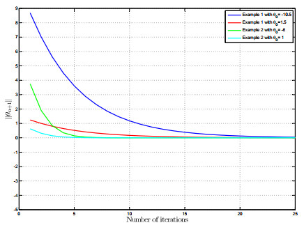
Figure 1.
Convergence behavior of {θn} for Example 3.1 and Example 3.2 with initial values θ0=−10.5,θ0=1.5, and θ0=−6,θ0=1, respectively.
This work focused on the investigation of a generalized variation inclusion problem. The resolvent operator for generalized η-co-monotone mapping was structured, the Lipschitz constant was estimated and its relationship with the graph convergence was accomplished. An Ishikawa type iterative algorithm was designed by incorporating the resolvent operator and total asymptotically non-expansive mapping. By employing the novel implication of graph convergence and analyzing the convergence of the considered iterative method, the common solution of the generalized variational inclusion and the set of fixed points of a total asymptotically non-expansive mapping was obtained. Moreover, a generalized resolvent dynamical system was investigated. Some of its attributes were discussed and implemented to examine the considered generalized variation inclusion problem.
Citation: Doaa Filali, Mohammad Dilshad, Mohammad Akram. Generalized variational inclusion: graph convergence and dynamical system approach[J]. AIMS Mathematics, 2024, 9(9): 24525-24545. doi: 10.3934/math.20241194
| [1] | Javid Iqbal, Imran Ali, Puneet Kumar Arora, Waseem Ali Mir . Set-valued variational inclusion problem with fuzzy mappings involving XOR-operation. AIMS Mathematics, 2021, 6(4): 3288-3304. doi: 10.3934/math.2021197 |
| [2] | Jamilu Abubakar, Poom Kumam, Jitsupa Deepho . Multistep hybrid viscosity method for split monotone variational inclusion and fixed point problems in Hilbert spaces. AIMS Mathematics, 2020, 5(6): 5969-5992. doi: 10.3934/math.2020382 |
| [3] | Yali Zhao, Qixin Dong, Xiaoqing Huang . A self-adaptive viscosity-type inertial algorithm for common solutions of generalized split variational inclusion and paramonotone equilibrium problem. AIMS Mathematics, 2025, 10(2): 4504-4523. doi: 10.3934/math.2025208 |
| [4] | Iqbal Ahmad, Mohd Sarfaraz, Syed Shakaib Irfan . Common solutions to some extended system of fuzzy ordered variational inclusions and fixed point problems. AIMS Mathematics, 2023, 8(8): 18088-18110. doi: 10.3934/math.2023919 |
| [5] | Yasir Arfat, Supak Phiangsungnoen, Poom Kumam, Muhammad Aqeel Ahmad Khan, Jamshad Ahmad . Some variant of Tseng splitting method with accelerated Visco-Cesaro means for monotone inclusion problems. AIMS Mathematics, 2023, 8(10): 24590-24608. doi: 10.3934/math.20231254 |
| [6] | Feng Ma, Bangjie Li, Zeyan Wang, Yaxiong Li, Lefei Pan . A prediction-correction based proximal method for monotone variational inequalities with linear constraints. AIMS Mathematics, 2023, 8(8): 18295-18313. doi: 10.3934/math.2023930 |
| [7] | Yunda Dong, Yiyi Li . A new operator splitting method with application to feature selection. AIMS Mathematics, 2025, 10(5): 10740-10763. doi: 10.3934/math.2025488 |
| [8] | Mohammad Dilshad, Aysha Khan, Mohammad Akram . Splitting type viscosity methods for inclusion and fixed point problems on Hadamard manifolds. AIMS Mathematics, 2021, 6(5): 5205-5221. doi: 10.3934/math.2021309 |
| [9] | Iqbal Ahmad, Faizan Ahmad Khan, Arvind Kumar Rajpoot, Mohammed Ahmed Osman Tom, Rais Ahmad . Convergence analysis of general parallel $ S $-iteration process for system of mixed generalized Cayley variational inclusions. AIMS Mathematics, 2022, 7(11): 20259-20274. doi: 10.3934/math.20221109 |
| [10] | Mohammad Dilshad, Fahad Maqbul Alamrani, Ahmed Alamer, Esmail Alshaban, Maryam G. Alshehri . Viscosity-type inertial iterative methods for variational inclusion and fixed point problems. AIMS Mathematics, 2024, 9(7): 18553-18573. doi: 10.3934/math.2024903 |
This work focused on the investigation of a generalized variation inclusion problem. The resolvent operator for generalized η-co-monotone mapping was structured, the Lipschitz constant was estimated and its relationship with the graph convergence was accomplished. An Ishikawa type iterative algorithm was designed by incorporating the resolvent operator and total asymptotically non-expansive mapping. By employing the novel implication of graph convergence and analyzing the convergence of the considered iterative method, the common solution of the generalized variational inclusion and the set of fixed points of a total asymptotically non-expansive mapping was obtained. Moreover, a generalized resolvent dynamical system was investigated. Some of its attributes were discussed and implemented to examine the considered generalized variation inclusion problem.
The theory of variational inequalities (VIs) was initially originated from variational principles for investigating partial differential equations [31]. It is a dynamic tool for unifying and studying equilibrium problems. It has been recognized as a potential and compelling approach for exploring and analyzing nonlinear problems of science and engineering, complex boundary value problems, models of economics, and transportation and operations research by reformatting them as a VI. Since its rise, this theory has been augmented by diverse techniques and methodologies.
Among the succeeding expansions, one of the prominent, most fruitful and worthwhile generalizations of VI is variational inclusion. The variational inclusion problem plays a crucial role in the formulation of mathematical models of various real-life problems with practical implications across diverse disciplines. The monotone inclusion problem (MIP) is to discern an element θ∗∈H so that
| 0∈(φ+ψ)θ∗, | (1.1) |
where H is a real Hilbert space, ψ:H→H is a single-valued monotone operator, and φ:H→2H is a maximal monotone operator. We indicate the solution set of the MIP (1.1) by (φ+ψ)−1(0). Variational inclusions have been implemented to tackle numerous equilibrium and optimization problems including image processing, image deblurring, convex minimization, DC programming, split feasibility, fixed point and VI problems; see [1,9,12,17,21,23,27,28,29,33]. Applicability and usefulness of variational inclusions have captivated the attentiveness of numerous scholars in a short span of time. As of now, a number of approaches have been carried out for figuring out the problem. One of the fundamental approaches to deal with these problems is to reduce the inclusion problem into an analogous fixed point problem by employing the technique of resolvent.
In recent times, for the sake of generalizing VIs and inclusions, the researchers have generalized the conception of monotone and accretive mappings such as m-accretive mappings [20] as an allied approach for maximal monotone, maximal η-monotone and η-subdifferential mappings. In this sequel, the concept of H-monotone mapping was incepted by Fang and Huang [15] in Hilbert spaces, and later they further coined an analogous notion in Banach spaces named H-accretive mappings [16]. In 2008, Zou and Huang [35] enriched the literature by defining the H(⋅,⋅)-accretive operator in Banach spaces. Using these generalized monotone and accretive mappings, authors have examined numerous variational inclusions by implementing the resolvent operators. Moreover, the notion of the H(⋅,⋅)-co-coercive mapping was set forth by Ahmad et al. [3]. This concept was further extended by defining H(⋅,⋅)-co-monotone mapping [4], which is the combination of symmetric co-coercive and monotone mapping. An analogous conception was studied in Banach spaces and named as H(⋅,⋅)-co-accretive mapping [5], which is the combination of symmetric co-coercive and accretive mapping. The researchers explored some properties of these operators and applied them to investigate a number of variational inclusions. Subsequently, a great deal of work has gone into examining variational inclusion problems involving generalized monotone and accretive mappings using the graph convergence. Li and Huang [22] brought the idea of graph convergence for H(⋅,⋅)-accretive mappings and shown that it is homologous to the resolvent operator convergence Further, Ahmad et al. [2] utilized the conception of graph convergence to examine a system of generalized variational inclusions involving H(⋅,⋅)-co-accretive mapping. For a detailed literature on graph convergence, we refer to [6,7,10,32].
Since the equilibrium point of the dynamical system leads to the solution of the corresponding VI and inclusion problem, dynamical systems represent cohesive, all-encompassing frameworks of VIs and inclusions as their equilibrium points serve as solutions to these problems. Thus, all the problems whose mathematical models can be solved using VIs can also be examined in the general framework of the dynamical systems. This characteristic has drawn the attention of researchers to study dynamical systems associated with VI and inclusion problems. One can transform the model of VI or inclusion problems into a fixed point problem by implementing the novel resolvent or projection operator, and such transformations allow us to suggest dynamical systems. Dynamical systems directly or indirectly appear in several useful areas encompassing celestial mechanics, environmental studies, financial forecasting, modeling of neuroscience, etc., and allow us to describe the trajectories of physical process and real-world problems before achieving the steady state. For further applications of the dynamical systems, see [13,14,18,24,25,26].
Inspired and persuaded by the above stated work, in this study, we investigate a generalized variation inclusion problem. We define the resolvent operator for generalized η-co-monotone mapping and estimate its Lipschitz constant. Further, its relationship with the graph convergence is accomplished. An Ishikawa type iterative algorithm is structured and analyzed to obtain the common solution of the generalized variational inclusion and the set of fixed points of a total asymptotically non-expansive mapping by employing the novel implication of graph convergence. Moreover, we construct a generalized resolvent dynamical system associated to the generalized variational inclusion and discuss some of its attributes. Further, we investigated the considered generalized variation inclusion problem by implementing the generalized resolvent dynamical system. Also, the theoretical results are verified by illustrative examples.
Now onward, H is assumed to be a real Hilbert space endued with norm ‖⋅‖ which induces the metric d and inner product ⟨⋅,⋅⟩. The collection of all closed and bounded subsets of H is signified as CB(H).
Definition 2.1. Let η:H×H→H be a single-valued mapping. A mapping ψ:H→H is referred to as
(i) η-monotone if
| ⟨ψ(θ)−ψ(ϑ),η(θ,ϑ)⟩≥0,∀θ,ϑ∈H; |
(ii) ρ-strongly η-monotone if ∃ρ>0 so that
| ⟨ψ(θ)−ψ(ϑ),η(θ,ϑ)⟩≥ρ‖θ−ϑ‖2,∀θ,ϑ∈H; |
(iii) ϖ-Lipschitz continuous if ∃ϖ>0 so that
| ‖ψ(θ)−ψ(ϑ)‖≤ϖ‖θ−ϑ‖,∀θ,ϑ∈H; |
(iv) ζ-expansive if ∃ζ>0 so that
| ‖ψ(θ)−ψ(ϑ)‖≥ζ‖θ−ϑ‖,∀θ,ϑ∈H. |
The following lemma is a crucial instrument for carrying out the adopted scheme.
Lemma 2.1. [34] Let {pk}∞k=1 be a nonnegative real sequence and {qk}∞k=1 be a real sequence in [0, 1] with ∑∞k=0qk=∞ fulfilling the following inequality:
| pk+1≤(1−qk)pk+qkτk,∀k≥n0, |
where τk≥0,∀k≥0 and limk→∞τk=0. Then limk→∞pk=0.
Definition 2.2. Let η,Φ:H×H→H and ψ,φ:H→H be the single-valued mappings. Then Φ(⋅,⋅) is known as
(i) m-mixed Lipschitz continuous with respect to ψ and φ if ∃m>0 such that
| ‖Φ(ψ(θ),φ(θ))−Φ(ψ(ϑ),φ(ϑ))‖≤m‖θ−ϑ‖,∀θ,ϑ∈H; |
(ii) η-co-coercive with respect to ψ if ∃κ′>0 such that
| ⟨Φ(ψ(θ),a)−Φ(ψ(ϑ),a),η(θ,ϑ)⟩≥κ′‖ψ(θ)−ψ(ϑ)‖2,∀θ,ϑ∈H; |
(iii) relaxed η-co-coercive with respect to φ if ∃κ″>0 such that
| ⟨Φ(b,φ(θ))−Φ(b,φ(ϑ)),η(θ,ϑ)⟩≥(−κ″)‖φ(θ)−φ(ϑ)‖2,∀θ,ϑ∈H; |
(iv) symmetric η-co-coercive with respect to ψ and φ if Φ(⋅,⋅) satisfies (ii) and (iii).
Definition 2.3. Let η,Φ:H×H→H; G,ψ,φ:H→H be the single-valued mappings and Ψ:H→CB(H) be a set-valued mapping. Then, Φ(⋅,⋅) is known as mixed δ-strongly monotone with respect to G and Ψ, if for some ω∈Ψ(θ),ˉω∈Ψ(ϑ), ∃δ>0 such that
| ⟨Φ(ψ(θ),φ(θ))−Φ(ψ(ϑ),φ(ϑ)),η(G(ω),G(ˉω))⟩≥δ‖θ−ϑ‖2,∀θ,ϑ∈H. |
Definition 2.4. Let η:H×H→H and f,g:H→H be the single-valued mappings. A set-valued mapping M:H×H⇉H is known as
(i) τ′-strongly η-monotone with respect to f if ∃τ′>0 so that
| ⟨μ−ν,η(θ,ϑ)⟩≥τ′‖θ−ϑ‖2,∀θ,ϑ,b∈H,μ∈M(f(θ),b),ν∈M(f(ϑ),b); |
(ii) τ″-relaxed η-monotone with respect to g if ∃τ″>0 so that
| ⟨μ−ν,η(θ,ϑ)⟩≥(−τ″)‖θ−ϑ‖2,∀θ,ϑ,b∈H,μ∈M(b,g(θ)),ν∈M(b,g(ϑ)); |
(iii) M(⋅,⋅) is known as symmetric η-monotone with respect to f and g if M(⋅,⋅) satisfies (i) and (ii).
Definition 2.5. Let η,Φ:H×H→H and ψ,φ,f,g:H→H be the single-valued mappings. A set-valued mapping M:H×H⇉H is referred to as generalized η-co-monotone if Φ(⋅,⋅) is symmetric η-co-coercive with respect to ψ and φ, M(⋅,⋅) is symmetric η-monotone with respect to f and g, and
| [Φ(ψ,φ)+ϱM(f,g)](H)=H,∀ϱ>0. | (2.1) |
Note 2.1. Now onward, M is generalized η-co-monotone means, Φ(⋅,⋅) is η-symmetric co-coercive with respect to ψ and φ with constants κ′ and κ″, respectively, and M(⋅,⋅) is symmetric η-monotone with respect to f and g with constants τ′ and τ″, respectively, and satisfies (2.1).
Lemma 2.2. Let η,Φ:H×H→H and ψ,φ,f,g:H→H be the single-valued mappings. Let M:H×H⇉H be a generalized η-co-monotone mapping. Let ψ be ς-expansive and φ be l-Lipschitz continuous. Then, for all ϱ>0, the mapping [Φ(ψ,φ)+ϱM(f,g)]−1 is single-valued.
Definition 2.6. Let η,Φ:H×H→H and ψ,φ,f,g:H→H be the single-valued mappings. Let M:H×H⇉H be a generalized η-co-monotone mapping. The resolvent Rη,Φ(⋅,⋅)ϱ,M(⋅,⋅):H→H is described as
| Rη,Φ(⋅,⋅)ϱ,M(⋅,⋅)(θ)=[Φ(ψ,φ)+ϱM(f,g)]−1(θ),∀θ∈H,ϱ>0. | (2.2) |
Proposition 2.1. Let η:H×H→H be a π-Lipschitz continuous mapping; Φ:H×H→H and ψ,φ,f,g:H→H be the single-valued mappings such that ψ is ς-expansive and φ is l-Lipschitz continuous. Let M:H×H⇉H be a generalized η-co-monotone mapping. Then, Rη,Φ(⋅,⋅)ϱ,M(⋅,⋅):H→H is Ξ-Lipschitz continuous, where
| Ξ=π[ϱ(τ′−τ″)+(κ′ς2−κ″l2)]. |
Proof. For given θ,ϑ∈H, it follows from (2.2) that
| Rη,Φ(⋅,⋅)ϱ,M(⋅,⋅)(θ)=[Φ(ψ,φ)+ϱM(f,g)]−1(θ), | (2.3) |
| Rη,Φ(⋅,⋅)ϱ,M(⋅,⋅)(ϑ)=[Φ(ψ,φ)+ϱM(f,g)]−1(ϑ). | (2.4) |
From (2.3) and (2.4), one can write
| 1ϱ(θ−Φ(ψ(Rη,Φ(⋅,⋅)ϱ,M(⋅,⋅)(θ)),φ(Rη,Φ(⋅,⋅)ϱ,M(⋅,⋅)(θ))))∈M(f(Rη,Φ(⋅,⋅)ϱ,M(⋅,⋅)(θ)),g(Rη,Φ(⋅,⋅)ϱ,M(⋅,⋅)(θ))), | (2.5) |
| 1ϱ(ϑ−Φ(ψ(Rη,Φ(⋅,⋅)ϱ,M(⋅,⋅)(ϑ)),φ(Rη,Φ(⋅,⋅)ϱ,M(⋅,⋅)(ϑ))))∈M(f(Rη,Φ(⋅,⋅)ϱ,M(⋅,⋅)(ϑ)),g(Rη,Φ(⋅,⋅)ϱ,M(⋅,⋅)(ϑ))). | (2.6) |
For the sake of simplicity, we indicate Λ(θ)=Rη,Φ(⋅,⋅)ϱ,M(⋅,⋅)(θ) and Λ(ϑ)=Rη,Φ(⋅,⋅)ϱ,M(⋅,⋅)(ϑ), and since M(⋅,⋅) is symmetric η-monotone, then
| ϱ(τ′−τ″)‖Λ(θ)−Λ(ϑ)‖2≤⟨θ−Φ(ψ(Λ(θ)),φ(Λ(θ)))−(ϑ−Φ(ψ(Λ(ϑ)),φ(Λ(ϑ))),η(Λ(θ),Λ(ϑ))⟩≤⟨θ−ϑ,η(Λ(θ),Λ(ϑ))⟩−⟨Φ(ψ(Λ(θ)),φ(Λ(θ)))−Φ(ψ(Λ(ϑ)),φ(Λ(ϑ))),η(Λ(θ),Λ(ϑ))⟩=⟨θ−ϑ,η(Λ(θ),Λ(ϑ))⟩−⟨Φ(ψ(Λ(θ)),φ(Λ(θ)))−Φ(ψ(Λ(ϑ)),φ(Λ(θ))),η(Λ(θ),Λ(ϑ))⟩−⟨Φ(ψ(Λ(ϑ)),φ(Λ(θ)))−Φ(ψ(Λ(ϑ)),φ(Λ(ϑ))),η(Λ(θ),Λ(ϑ))⟩. |
Invoking symmetric η-co-coercivity of Φ, ς-expansiveness of ψ, l and π-Lipschitz continuities of φ and η, respectively, we attain ϱ(τ′−τ″)‖Λ(θ)−Λ(ϑ)‖2≤⟨θ−ϑ,η(Λ(θ),Λ(ϑ))⟩−(κ′ς2−κ″l2)‖Λ(θ)−Λ(ϑ)‖2, i.e.,
| [ϱ(τ′−τ″)+(κ′ς2−κ″l2)]‖Λ(θ)−Λ(ϑ)‖2≤‖θ−ϑ‖‖η(Λ(θ),Λ(ϑ))‖≤‖θ−ϑ‖π‖Λ(θ)−Λ(ϑ)‖. |
Thus, for all θ,ϑ∈H, we obtain ‖Λ(θ)−Λ(ϑ)‖≤Ξ‖θ−ϑ‖, i.e.,
| ‖Rη,Φ(⋅,⋅)ϱ,M(⋅,⋅)(θ)−Rη,Φ(⋅,⋅)ϱ,M(⋅,⋅)(ϑ)‖≤Ξ‖θ−ϑ‖,∀θ,ϑ∈H, | (2.7) |
where, Ξ=π[ϱ(τ′−τ″)+(κ′ς2−κ″l2)].
Definition 2.7. The graph of a multivalued mapping M:H×H⇉H is expressed as
| Graph(M)={((θ,ϑ),ξ):ξ∈M(θ,ϑ)}. |
Definition 2.8. Let η,Φ:H×H→H and ψ,φ,f,g:H→H be the single-valued mappings. For n≥0, let Mn,M:H×H⇉H be generalized η-co-monotone mappings. Then, {Mn}∞n=1 is known as graph convergent to M, indicated by (MnG→M) if for each (f(θ),g(θ),ξ)∈Graph(M), ∃{(f(θn),g(θn),ξn)}∈Graph(Mn) so that
| f(θn)→f(θ),g(θn)→g(θ)andξn→ξasn→∞. |
Theorem 2.1. Let η,Φ:H×H→H and ψ,φ,f,g:H→H be the single-valued mappings such that Φ(⋅,⋅) is m-mixed Lipschitz continuous with respect to ψ and φ, and f,g are continuous mappings so that f is ζ-expansive. For n≥0, let Mn,M:H×H⇉H be generalized η-co-monotone mappings. Then,
| MnG→M⇔Rη,Φ(⋅,⋅)ϱ,Mn(⋅,⋅)(θ)→Rη,Φ(⋅,⋅)ϱ,M(⋅,⋅)(θ),∀θ∈H,ϱ>0. |
Proof. For all θ∈H and ϱ>0, suppose that Rη,Φ(⋅,⋅)ϱ,Mn(⋅,⋅)(θ)→Rη,Φ(⋅,⋅)ϱ,M(⋅,⋅)(θ). Assume that (f(θ),g(θ),ξ)∈Graph(M), then
| θ=Rη,Φ(⋅,⋅)ϱ,M(⋅,⋅)[Φ(ψ(θ),φ(θ))+ϱξ]. | (2.8) |
Letting
| θn=Rη,Φ(⋅,⋅)ϱ,Mn(⋅,⋅)[Φ(ψ(θ),φ(θ))+ϱξ], | (2.9) |
which turns into
| Φ(ψ(θ),φ(θ))+ϱξ∈[Φ(ψ(θn),φ(θn))+ϱM(f(θn),g(θn))]. | (2.10) |
For each n≥0, take ξn∈M(f(θn),g(θn)), then (2.10) yields
| Φ(ψ(θ),φ(θ))+ϱξ=Φ(ψ(θn),φ(θn))+ϱξn. | (2.11) |
Invoking the m-mixed Lipschitz continuity of Φ, it follows from (2.11) that
| ‖ϱξn−ϱξ‖=‖Φ(ψ(θn),φ(θn))−Φ(ψ(θ),φ(θ))‖≤(ρ′+ρ″)‖θn−θ‖. | (2.12) |
Thus, ‖ξn−ξ‖≤mϱ‖θn−θ‖. Recalling the hypothesis Rη,Φ(⋅,⋅)ϱ,Mn(⋅,⋅)(θ)→Rη,Φ(⋅,⋅)ϱ,M(⋅,⋅)(θ), it yields from (2.8) and (2.9) that ‖θn−θ‖→0 and, hence, from (2.12), we acquire ‖ξn−ξ‖→0 as n→∞. Accounting the continuity of f and g, we deduce f(θn)→f(θ) and g(θn)→g(θ), and so MnG→M.
On the contrary, assume that MnG→M and choose an arbitrary but fixed e∈H. Since M(⋅,⋅) is a generalized η-co-monotone mapping, Range[Φ(ψ,φ)+ϱM(f,g)]=H. Then, there exists ((f(θ),g(θ)),ξ)∈Graph(M) such that e=Φ(ψ(θ),φ(θ))+ϱξ. Since (f(θ),g(θ),ξ)∈Graph(M) and suppose (f(θn),g(θn),ξn)∈Graph(Mn),
| θ=Rη,Φ(⋅,⋅)ϱ,M(⋅,⋅)[Φ(ψ(θ),φ(θ))+ϱξ]andθn=Rη,Φ(⋅,⋅)ϱ,Mn(⋅,⋅)[Φ(ψ(θn),φ(θn))+ϱξn]. |
Letting en=Φ(ψ(θn),φ(θn))+ϱξn, for all n≥0, adducing the m-mixed Lipschitz continuity Φ(⋅,⋅) and making use of (2.7), we acquire
| ‖Rη,Φ(⋅,⋅)ϱ,Mn(⋅,⋅)(e)−Rη,Φ(⋅,⋅)ϱ,M(⋅,⋅)(e)‖ ≤‖Rη,Φ(⋅,⋅)ϱ,Mn(⋅,⋅)(e)−Rη,Φ(⋅,⋅)ϱ,Mn(⋅,⋅)(en)‖+‖Rη,Φ(⋅,⋅)ϱ,Mn(⋅,⋅)(en)−Rη,Φ(⋅,⋅)ϱ,M(⋅,⋅)(e)‖≤Ξ‖en−e‖+‖θn−θ‖=Ξ‖Φ(ψ(θn),φ(θn))+ϱξn−[Φ(ψ(θ),φ(θ))+ϱξ]‖+‖θn−θ‖≤Ξ‖Φ(ψ(θn),φ(θn))−Φ(ψ(θ),φ(θ))‖+Ξϱ‖ξn−ξ‖+‖θn−θ‖≤[1+Ξm]‖θn−θ‖+Ξϱ‖ξn−ξ‖. | (2.13) |
The ζ-expansiveness of f yields
| ‖f(θn)−f(θ)‖≥ζ‖θn−θ‖≥0. | (2.14) |
Thus, we deduce from (2.14) and the Definition 2.8 that θn→θ and ξn→ξ as n→∞. Thus, from (2.13), we infer that Rη,Φ(⋅,⋅)ϱ,Mn(⋅,⋅)(θ)→Rη,Φ(⋅,⋅)ϱ,M(⋅,⋅)(θ).
Example 2.1 Let H=R2 with the usual inner product on R2, i.e.,
| ⟨(θ1,θ2),(ϑ1,ϑ2)⟩=θ1ϑ1+θ2ϑ2,∀(θ1,θ2),(ϑ1,ϑ2)∈R2. |
Define ψ,φ:R2→R2 and η,Φ:R2×R2→R2 by
| ψ(θ1,θ2)=(θ14,θ22),φ(θ1,θ2)=(−θ12,−2θ23),∀(θ1,θ2)∈R2,Φ(ψ(θ),φ(θ))=ψ(θ)+φ(θ),∀θ∈R2,η(θ,ϑ)=θ−ϑ2,∀θ,ϑ∈R2. |
Then, for any fixed ς∈R2, we find
| ⟨Φ(ψ(θ),ς)−Φ(ψ(ϑ),ς),η(θ,ϑ)⟩≥1‖ψ(θ)−ψ(ϑ)‖2,⟨Φ(ς,φ(θ))−Φ(ς,φ(ϑ)),η(θ,ϑ)⟩≥(−1)‖φ(θ)−φ(ϑ)‖2. |
Thus, Φ(⋅,⋅) is η-co-coercive with respect to ψ and relaxed η-co-coercive with respect to φ, hence Φ(⋅,⋅) is symmetric η-co-coercive. Next, we estimate the symmetric monotonicity of M. Define f,g:R2→R2 and M:R2×R2→R2 by
| f(θ1,θ2)=(θ13−θ2,θ1+θ22),g(θ1,θ2)=(θ13+θ22,−θ12+θ24),∀(θ1,θ2)∈R2,M(f(θ),g(θ))=f(θ)−g(θ),∀θ∈R2. |
Then for any fixed ϖ∈R2, we find
| ⟨M(f(θ),ϖ)−M(f(ϑ),ϖ),η(θ,ϑ)⟩≥16‖θ−ϑ‖2,⟨M(ϖ,g(θ))−M(ϖ,g(ϑ)),η(θ,ϑ)⟩≥−16‖θ−ϑ‖2, |
i.e., M(⋅,⋅) is η-monotone with respect to f and relaxed η-monotone with respect to g, hence M(⋅,⋅) is symmetric η-monotone. Also, for any θ∈R2 and ϱ>0,
| [Φ(ψ,φ)+ϱM(f,g)](θ)=ψ(θ)+φ(θ)+ϱ(f(θ)−g(θ))=[−θ14−3ϱ2θ2,3ϱ2θ1+(ϱ4−16)θ2], |
i.e., [Φ(ψ,φ)+ϱM(f,g)](R2)=R2,∀ϱ>0. Thus, M(⋅,⋅) is a generalized η-co-monotone mapping. Further, we show that MnG→M. Let
| f(θn)=(θ13−θ2+2n,θ1+θ22+1n),g(θn)=(θ13+θ22+2n2,−θ12+θ24+1n2), |
and ξn=Mn(f(θn),g(θn))=f(θn)−g(θn)=(−32θ2+2n−2n2,32θ1+14θ2+1n−1n2). One can observe that
| limn→∞f(θn)=limn→∞(θ13−θ2+2n,θ1+θ22+1n)=(θ13−θ2,θ1+θ22),limn→∞g(θn)=limn→∞(θ13+θ22+2n2,−θ12+θ24+1n2)=(θ13+θ22,−θ12+θ24), |
and limn→∞ξn=limn→∞(−32θ2+2n−2n2,32θ1+14θ2+1n−1n2)=f(θ)−g(θ)=M(f(θ),g(θ))=ξ.
Thus, we acquire that limn→∞f(θn)=f(θ) and limn→∞g(θn)=g(θ) and limn→∞ξn=ξ. Hence, MnG→M. Finally, it remains to manifest that MnG→M⇔Rη,Φ(⋅,⋅)ϱ,Mn(⋅,⋅)(θ)→Rη,Φ(⋅,⋅)ϱ,M(⋅,⋅)(θ),∀θ∈H,ϱ>0. Now, for ϱ=1, the associated resolvent operators are estimated as:
| Rη,Φ(⋅,⋅)ϱ,Mn(⋅,⋅)(θ)=[Φ(ψ,φ)+Mn(f,g)]−1(θ)=(−14θ1−32θ2+2n−2n2,32θ1+112θ2+1n−1n2)−1=1107(4θ1+72θ2−80n+80n2,−72θ1−12θ2+156n−156n2) |
and
| Rη,Φ(⋅,⋅)ϱ,M(⋅,⋅)(θ)=[Φ(ψ,φ)+M(f,g)]−1(θ)=(−14θ1−32θ2,32θ1+112θ2)−1=1107(4θ1+72θ2,−72θ1−12θ2), |
which yields
| ‖Rη,Φ(⋅,⋅)ϱ,Mn(⋅,⋅)(θ)−Rη,Φ(⋅,⋅)ϱ,(⋅,⋅)(θ)‖→0asn→∞. |
Thus, we obtain
| ‖Rη,Φ(⋅,⋅)ϱ,Mn(⋅,⋅)(θ)→Rη,Φ(⋅,⋅)ϱ,(⋅,⋅)(θ)‖asMnG→M. |
In this section, we employ a generalized η-co-monotone mapping for investigating a general variational inclusion (GVIP). We examine the problem of discerning θ∈H,ω∈Ψ(θ) so that
| 0∈G(ω)+M(f(θ),g(θ)), | (3.1) |
where G,f,g:H→H and M:H×H⇉H;Ψ:H⇉CB(H) are single-valued and multivalued mappings, respectively. We signify the Problem (3.1) as GVIP and its solution set by Ω(H,M,Φ,G,η).
Lemma 3.1. Let η,Φ:H×H→H and G,ψ,φ,f,g:H→H be the single-valued mappings and Ψ:H⇉CB(H) a multivalued mapping. Let M:H×H⇉H be a generalized η-co-monotone mapping. Then, (θ,ω), where θ∈H,ω∈Ψ(θ) solves GVIP (3.1) if, and only if,
| θ=Rη,Φ(⋅,⋅)ϱ,M(⋅,⋅)[Φ(ψ(θ),φ(θ))−ϱG(ω)]. | (3.2) |
Proof. One can obtain the conclusion immediately by implementing (2.2).
A mapping F:H→H is referred to as non-expansive (NM) if ‖F(θ)−F(ϑ)‖≤‖θ−ϑ‖,∀θ,ϑ∈H. In [19], the authors defined a generalized NM referred to as asymptotically nonexpansive (ANM) which properly includes the class of NM.
Definition 3.1. [19] A mapping F:H→H is known as ANM if ∃ is a sequence {εn}⊆[1,∞) with limn→∞εn=1 and ∀n∈N,
| ‖Fn(θ)−Fn(ϑ)‖≤εn‖θ−ϑ‖,∀θ,ϑ∈H. |
In an attempt to obtain extension of NM and ANM, Sahu [30] introduced nearly asymptotically non-expansive mapping (NANM). The class of NANM is an intermediate class which contains the class of ANM and is contained in the class of mappings of asymptotically non-expansive type.
Definition 3.2. A mapping F:H→H is known as NANM, if ∃{εn}⊆[1,∞) and {υn}⊆[0,∞) with limn→∞εn=1,limn→∞υn=0, ∀n∈N,
| ‖Fn(θ)−Fn(ϑ)‖≤εn‖θ−ϑ‖+υn,∀θ,ϑ∈H. |
Further, Alber et al. [8] made an attempt to unify some classes of generalized NMs by introducing total asymptotically non-expansive mapping (TANM).
Definition 3.3. A mapping F:H→H is known as TANM if ∃ nonnegative sequences of real numbers {εn},{υn} with limn→∞εn=0=limn→∞υn and a strictly increasing continuous function γ:R+→R+ such that γ(0)=0 and ∀n∈N,
| ‖Fn(θ)−Fn(ϑ)‖≤‖θ−ϑ‖+μnγ(‖θ−ϑ‖)+νn,∀θ,ϑ∈H. |
Let F:H→H be a TANM and presume that the mappings η,Φ,G,ψ,φ,f,g,Ψ, and M are identical as in Lemma 3.1. Suppose that θ∗∈Fix(F)∩Ω(H,M,Φ,G,η), then from (3.2), one can achieve the following formulation:
| θ∗=Fnθ∗=Rη,Φ(⋅,⋅)ϱ,M(⋅,⋅)[Φ(ψ(θ∗),φ(θ∗))−ϱG(ω∗)]=FnRη,Φ(⋅,⋅)ϱ,M(⋅,⋅)[Φ(ψ(θ∗),φ(θ∗))−ϱG(ω∗)], | (3.3) |
where ϱ>0 and ω∗∈Ψ(θ∗). By the virtue of formulation (3.3), we design the following Ishikawa type resolvent iterative scheme to explore a common element of Fix(F) and Ω(H,M,Φ,G,η). Here, Fix(F) indicates the set of fixed points of TANM F and Ω(H,M,Φ,G,η) indicates the solution set of GVIP (3.1).
Algorithm 3.1. Let η,Φ:H×H→H and G,ψ,φ,f,g:H→H be the single-valued mappings. Let Ψ:H⇉CB(H) be a multivalued mapping; Mn,M:H×H⇉H be generalized η-co-monotone mappings, and F:H→H be a TANM. For initial points θ0,ϑ0∈H,ω0∈Ψ(θ0), estimate the sequences {θn},{ωn} by the following procedure:
| θn+1=(1−αn)θn+αnFnRη,Φ(⋅,⋅)ϱ,Mn(⋅,⋅)[Φ(ψ(ϑn),φ(ϑn))−ϱG(ˉωn)], | (3.4) |
| ϑn=(1−βn)θn+βnFnRη,Φ(⋅,⋅)ϱ,Mn(⋅,⋅)[Φ(ψ(θn),φ(θn))−ϱG(ωn)], | (3.5) |
for n=0,1,2,⋯, ωn∈Ψ(θn),ˉωn∈Ψ(ϑn), 0≤αn,βn≤1,∞∑n=0αn=∞, and ϱ>0.
Theorem 3.1. Let η:H×H→H be a π-Lipschitz continuous mapping; Φ:H×H→H and ψ,φ,f,g:H→H be the single-valued mappings such that Φ(⋅,⋅) is m-mixed Lipschitz continuous with respect to ψ and φ and ι-mixed strongly monotone with respect to G and Ψ, G is t-Lipschitz continuous, Ψ is D-Lipschitz continuous with constant r, ψ is ς-expansive, and φ is l-Lipschitz continuous. Let Mn,M:H×H⇉H be generalized η-co-monotone mappings. Let F:H→H be a ({μn},{νn},ϕ)-TANM so that Fix(F)∩Ω(H,M,Φ,G,η)≠∅. If ϱ>0 obeys the following relation:
| √m2−2ϱι+ϱ2t2r2<[ϱ(τ′−τ″)+(κ′ς2−κ″l2)]π. | (3.6) |
(i) Then Ω(H,M,Φ,G,η) is singleton.
(ii) If MnG→M, then the sequence {θn} induced by (3.4)-(3.5) converges strongly to θ∈Fix(F)∩Ω(H,M,Φ,G,η).
Proof. (i) Define G:H→H as
| G(θ)=Rη,Φ(⋅,⋅)ϱ,M(⋅,⋅)[Φ(ψ(θ),φ(θ))−ϱG(ω)],∀θ∈H. | (3.7) |
By making use of Proposition 2.1 and (3.7), for all θ,ϑ∈H, we acquire
| ‖G(θ)−G(ϑ)‖=‖Rη,Φ(⋅,⋅)ϱ,M(⋅,⋅)[Φ(ψ(θ),φ(θ))−ϱG(ω)]−Rη,Φ(⋅,⋅)ϱ,M(⋅,⋅)[Φ(ψ(ϑ),φ(ϑ))−ϱG(ˉω)]‖≤Ξ‖Φ(ψ(θ),φ(θ))−Φ(ψ(ϑ),φ(ϑ))−ϱ(G(ω)−ϱG(ˉω))‖. | (3.8) |
Utilizing the m-mixed Lipschitz continuity and ι-mixed strong monotonicity of Φ and Lipschitz continuities of G and Ψ, we acquire
| ‖Φ(ψ(θ),φ(θ))−Φ(ψ(ϑ),φ(ϑ))−ϱ(G(ω)−ϱG(ˉω))‖2=‖Φ(ψ(θ),φ(θ))−Φ(ψ(ϑ),φ(ϑ))‖2−2ϱ⟨Φ(ψ(θ),φ(θ))−Φ(ψ(ϑ),φ(ϑ)),G(ω)−G(ˉω)⟩+ϱ2‖G(ω)−G(ˉω)‖2≤(m2−2ϱι+ϱ2t2r2)‖θ−ϑ‖2. | (3.9) |
After simplification, the above inequality turns into
| ‖Φ(ψ(θ),φ(θ))−Φ(ψ(ϑ),φ(ϑ))−ϱ(G(ω)−ϱG(ˉω))‖≤√m2−2ϱι+ϱ2t2r2‖θ−ϑ‖. | (3.10) |
Thus, (3.10) and (3.8) yield
| ‖G(θ)−G(ϑ)‖≤Θ‖θ−ϑ‖, | (3.11) |
where Θ=Ξ√m2−2ϱι+ϱ2t2r2 and Ξ=π[ϱ(τ′−τ″)+(κ′ς2−κ″l2)]. Taking the premise (3.6) into consideration, we see that 0≤Θ<1. Thus, G being a contraction mapping owns a unique fixed point, i.e., ∃ a unique θ∈H so that Rη,Φ(⋅,⋅)ϱ,M(⋅,⋅)[Φ(ψ(θ),φ(θ))−ϱG(ω)]=θ. Consequently, Lemma 3.1 guarantees that Ω(H,M,Φ,G,η) is singleton.
(ii) By the assumption that ∅≠Fix(F)∩Ω(H,M,Φ,G,η) and in (i), we confirmed that Ω(H,M,Φ,G,η) is singleton. Suppose that Ω(H,M,Φ,G,η)={θ}, then we deduce that θ∈Fix(F) and consequently, by (3.3), one can express
| θ=(1−αn)θ+αnFnRη,Φ(⋅,⋅)ϱ,M(⋅,⋅)[Φ(ψ(ϑ),φ(ϑ))−ϱG(ˉω)]]=(1−βn)θ+βnFnRη,Φ(⋅,⋅)ϱ,M(⋅,⋅)[Φ(ψ(θ),φ(θ))−ϱG(ω)]. | (3.12) |
Utilizing the Proposition 2.1, we get
| ‖Rη,Φ(⋅,⋅)ϱ,Mn(⋅,⋅)[Φ(ψ(ϑn),φ(ϑn))−ϱG(ˉωn)]−Rη,Φ(⋅,⋅)ϱ,M(⋅,⋅)[Φ(ψ(θ),φ(θ))−ϱG(ω)]‖≤‖Rη,Φ(⋅,⋅)ϱ,Mn(⋅,⋅)[Φ(ψ(ϑn),φ(ϑn))−ϱG(ˉωn)]−Rη,Φ(⋅,⋅)ϱ,Mn(⋅,⋅)[Φ(ψ(θ),φ(θ))−ϱG(ω)]‖+‖Rη,Φ(⋅,⋅)ϱ,Mn(⋅,⋅)[Φ(ψ(θ),φ(θ))−ϱG(ω)]−Rη,Φ(⋅,⋅)ϱ,M(⋅,⋅)[Φ(ψ(θ),φ(θ))−ϱG(ω)]‖≤Ξ‖Φ(ψ(ϑn),φ(ϑn))−ϱG(ˉωn)−[Φ(ψ(θ),φ(θ))−ϱG(ω)]‖+‖Σn‖=Ξ‖Φ(ψ(ϑn),φ(ϑn))−Φ(ψ(θ),φ(θ))−ϱ[G(ˉωn)−G(ω)]‖+‖Σn‖, | (3.13) |
where Σn=Rη,Φ(⋅,⋅)ϱ,Mn(⋅,⋅)[Φ(ψ(θ),φ(θ))−ϱG(ω)]−Rη,Φ(⋅,⋅)ϱ,M(⋅,⋅)[Φ(ψ(θ),φ(θ))−ϱG(ω)]. Utilizing the Lipschtz continuities of Ψ and G, we acquire
| ‖G(ˉωn)−G(ω)‖≤t‖ˉωn−ω‖≤tD(Ψ(ˉωn),Ψ(ω))≤tr‖ϑn−θ‖. | (3.14) |
Also, utilizing m-mixed Lipschitz continuity of Φ regarding ψ and φ, ι-mixed strong monotonicity with respect to G and Ψ and combining (3.14), we acquire
| ‖Φ(ψ(ϑn),φ(ϑn))−Φ(ψ(θ),φ(θ))−ϱ[G(ˉωn)−G(ω)]‖2=‖Φ(ψ(ϑn),φ(ϑn))−Φ(ψ(θ),φ(θ))‖2−2ϱ⟨Φ(ψ(ϑn),φ(ϑn))−Φ(ψ(θ),φ(θ)),G(ˉωn)−G(ω)⟩+ϱ2‖G(ˉωn)−G(ω)‖2≤m2‖ϑn−θ‖2−2ϱι‖ϑn−θ‖2+ϱ2t2r2‖ϑn−θ‖2=(m2−2ϱι+ϱ2t2r2)‖ϑn−θ‖2, |
which yields
| ‖Φ(ψ(ϑn),φ(ϑn))−Φ(ψ(θ),φ(θ))−ϱ[G(ˉωn)−G(ω)]‖≤√m2−2ϱι+ϱ2t2r2‖ϑn−θ‖. | (3.15) |
After substituting (3.15) into (3.13), we obtain
| ‖Rη,Φ(⋅,⋅)ϱ,Mn(⋅,⋅)[Φ(ψ(ϑn),φ(ϑn))−ϱG(ˉωn)]−Rη,Φ(⋅,⋅)ϱ,M(⋅,⋅)[Φ(ψ(θ),φ(θ))−ϱG(ω)]‖≤Θ‖ϑn−θ‖+‖Σn‖, | (3.16) |
where Θ=Ξ√m2−2ϱι+ϱ2t2r2. Now, recalling that F is ({μn},{νn},ϕ)-total asymptotically non-expansive and applying (3.4) and (3.12), we get
| ‖θn+1−θ‖=‖(1−αn)θn+αnFnRη,Φ(⋅,⋅)ϱ,Mn(⋅,⋅)[Φ(ψ(ϑn),φ(ϑn))−ϱG(ˉωn)]−[(1−αn)θ+αnFnRη,Φ(⋅,⋅)ϱ,M(⋅,⋅)[Φ(ψ(θ),φ(θ))−ϱG(ω)]]‖≤(1−αn)‖θn−θ‖+αn‖FnRη,Φ(⋅,⋅)ϱ,Mn(⋅,⋅)[Φ(ψ(ϑn),φ(ϑn))−ϱG(ˉωn)]−FnRη,Φ(⋅,⋅)ϱ,M(⋅,⋅)[Φ(ψ(θ),φ(θ))−ϱG(ω)]‖≤(1−αn)‖θn−θ‖+αn[‖Rη,Φ(⋅,⋅)ϱ,Mn(⋅,⋅)[Φ(ψ(ϑn),φ(ϑn))−ϱG(ˉωn)]−Rη,Φ(⋅,⋅)ϱ,M(⋅,⋅)[Φ(ψ(θ),φ(θ))−ϱG(ω)]‖+μnϕ[‖Rη,Φ(⋅,⋅)ϱ,Mn(⋅,⋅)[Φ(ψ(ϑn),φ(ϑn))−ϱG(ˉωn)]−Rη,Φ(⋅,⋅)ϱ,M(⋅,⋅)[Φ(ψ(θ),φ(θ))−ϱG(ω)]‖]+νn]. | (3.17) |
By substituting (3.16) in (3.17), we acquire
| ‖θn+1−θ‖≤(1−αn)‖θn−θ‖+αn[(Θ‖ϑn−θ‖+‖Σn‖)+μnϕ(Θ‖ϑn−θ‖+‖Σn‖)+νn]. | (3.18) |
Following the same steps and employing the same facts as in (3.17), it follows from (3.5) and (3.12) that
| ‖ϑn−θ‖=‖(1−βn)θn+βnFnRη,Φ(⋅,⋅)ϱ,Mn(⋅,⋅)[Φ(ψ(θn),φ(θn))−ϱG(ωn)]−[(1−βn)θ+βnFnRη,Φ(⋅,⋅)ϱ,M(⋅,⋅)[Φ(ψ(θ),φ(θ))−ϱG(ω)]]‖≤(1−βn)‖θn−θ‖+βn‖FnRη,Φ(⋅,⋅)ϱ,Mn(⋅,⋅)[Φ(ψ(θn),φ(θn))−ϱG(ωn)]−FnRη,Φ(⋅,⋅)ϱ,M(⋅,⋅)[Φ(ψ(θ),φ(θ))−ϱG(ω)]‖≤(1−βn)‖θn−θ‖+βn[‖Rη,Φ(⋅,⋅)ϱ,Mn(⋅,⋅)[Φ(ψ(θn),φ(θn))−ϱG(ωn)]−Rη,Φ(⋅,⋅)ϱ,M(⋅,⋅)[Φ(ψ(θ),φ(θ))−ϱG(ω)]‖+μnϕ[‖Rη,Φ(⋅,⋅)ϱ,Mn(⋅,⋅)[Φ(ψ(θn),φ(θn))−ϱG(ωn)]−Rη,Φ(⋅,⋅)ϱ,M(⋅,⋅)[Φ(ψ(θ),φ(θ))−ϱG(ω)]‖]+νn]≤(1−βn)‖θn−θ‖+βn[(Θ‖θn−θ‖+‖Σn‖)+μnϕ(Θ‖θn−θ‖+‖Σn‖)+νn]. | (3.19) |
By the hypothesis MnG→M, we obtain Σn→0, thus from (3.18) and (3.19), we deduce that
| ‖θn+1−θ‖≤(1−αn)‖θn−θ‖+αn[Θ‖ϑn−θ‖+μnϕ(Θ‖ϑn−θ‖)+νn]. | (3.20) |
| ‖ϑn−θ‖≤(1−βn)‖θn−θ‖+βn[Θ‖θn−θ‖+μnϕ(Θ‖θn−θ‖)+νn]. | (3.21) |
Substituting (3.21) into (3.20), we acquire
| ‖θn+1−θ‖≤(1−αn)‖θn−θ‖+αn[Θ{(1−βn)‖θn−θ‖+βn[Θ‖θn−θ‖+μnϕ(Θ‖θn−θ‖)+νn]}+μnϕ(Θ{(1−βn)‖θn−θ‖+βn[Θ‖θn−θ‖+μnϕ(Θ‖θn−θ‖)+νn]})+νn]=[(1−αn)+αnΘ[1−βn(1−Θ)]]‖θn−θ‖+αn[βnΘ{μnϕ(Θ‖θn−θ‖)+νn}+μnϕ{Θ{[1−βn(1−Θ)]‖θn−θ‖+μnϕ(Θ‖θn−θ‖)+νn}}+νn]≤[1−αn(1−Θ)]‖θn−θ‖+αn(1−Θ)[βnΘ{μnϕ(Ψn)+νn}+μnϕ{Θ{Γn+μnϕ(Ψn)+νn}}+νn](1−Θ), | (3.22) |
where Ψn=Θ‖θn−θ‖ and Γn=[1−βn(1−Θ)]‖θn−θ‖. For each n≥n0, setting pn=‖θn−θ‖,qn=αn(1−Θ) and τn=βnΘ[μnϕ(Ψn)+νn]+μnϕ[Θ{Γn+μnϕ(Ψn)+νn}]+νn(1−Θ). Clearly, ∑∞n=0qn=∞ because of ∑∞n=0αn=∞. In fact, μn,νn→0 as n→∞ yields τn=0. Thus, we deduce from Lemma 2.1 that limn→∞pn=0 and, hence, limn→∞θn=θ.
Example 3.1. Let H=[0,∞) with inner product ⟨θ,ϑ⟩=θϑ and norm |⋅|. Define F(θ)=sinθ,∀θ∈[0,∞). Then, clearly 0∈Fix(F) for all θ,ϑ∈[0,∞), and we express
| ‖F(θ)−F(ϑ)‖=‖sinθ−sinϑ‖=‖2sin(θ−ϑ)2⋅cos(θ+ϑ)2‖≤‖θ−ϑ‖. |
Thus, F is non-expansive, hence F is TANM with μn=1n2 and νn=1n3,∀n≥1. Define the mappings η,Φ:H×H→H and G,ψ,φ,f,g:H→H by
| η(θ,ϑ)=θ−ϑ4,Φ(ψ(θ),φ(θ))=ψ(θ)+φ(θ),G(θ)=θ−12,ψ(θ)=3θ+14,φ(θ)=−θ−14,f(θ)=4θ+1,g(θ)=−2θ+12. |
It can be easily observed that η,G, and φ are Lipschitz continuous with constants π=14,t=12, and φ=14, respectively, and ψ is 34-expansive. Also,
| ‖Φ(ψ(θ),φ(θ))−Φ(ψ(ϑ),φ(ϑ))‖≤12‖θ−ϑ‖,∀θ,ϑ∈H,⟨Φ(ψ(θ),φ(θ))−Φ(ψ(ϑ),φ(ϑ)),η(θ,ϑ)⟩≥18‖θ−ϑ‖2,∀θ,ϑ∈H,⟨Φ(ψ(θ),k)−Φ(ψ(ϑ),k),η(θ,ϑ)⟩≥13‖ψ(θ)−ψ(ϑ)‖2,∀θ,ϑ,k∈H,⟨Φ(k,φ(θ))−Φ(k,φ(ϑ)),η(θ,ϑ)⟩≥(−1)‖φ(θ)−φ(ϑ)‖2,∀θ,ϑ,k∈H, |
i.e., Φ(⋅,⋅) is 1/2-mixed Lipschitz continuous, 1/8-mixed strongly monotone, and symmetric η-co-coercive with respect to ψ and φ with constants 1/3 and 1, respectively. Define M:H×H⇉H and Ψ:H→CB(H) by M(f(θ),g(θ))=f(θ)+g(θ)3andΨ(θ)={θ5+1}. Then, Ψ is 1/5-Lipschitz continuous and
| ⟨M(f(θ),k)−M(f(ϑ),k),η(θ,ϑ)⟩≥1/3‖θ−ϑ‖2,∀θ,ϑ,k∈H,⟨M(k,g(θ))−M(k,g(ϑ)),η(θ,ϑ)⟩≥(−1/6)‖θ−ϑ‖2,∀θ,ϑ,k∈H, |
i.e., M(⋅,⋅) is symmetric η-monotone with respect to f and g with constants 1/3 and 1/6, respectively. Thus, M(⋅,⋅) is a generalized η-co-monotone mapping. Also, G(θ)=Rη,Φ(⋅,⋅)ϱ,M(⋅,⋅)[Φ(ψ(θ),φ(θ))−ϱG(ω)]=52θ and the estimated constants satisfy (3.6), that is, √m2−2ϱι+ϱ2t2r2<[ϱ(τ′−τ″)+(κ′ς2−κ″l2)]π. Therefore, θ∗=0∈H is a unique fixed point of G. Thus, we have θ∗=0∈Fix(F)∩Ω(H,M,Φ,G,η). Next, we compute the sequence {θn} by employing Algorithm 3.1. Let αn=n2n+1 and βn=1n+1. Then
| θn+1=(1−αn)θn+αnRη,Φ(⋅,⋅)ϱ,M(⋅,⋅)[Φ(ψ(ϑn),φ(ϑn))−ϱG(ˉωn)],θn+1=(n+12n+1)θn+(3n5(2n+1))ϑn,ϑn=(1−βn)θn+βnRη,Φ(⋅,⋅)ϱ,M(⋅,⋅)[Φ(ψ(θn),φ(θn))−ϱG(ωn)],ϑn=(nn+1)θn+(35(n+1))θn. |
For different initial points: θ0=−10.5 and θ0=1.5, the sequence θn→0 and 0∈Fix(F)∩Ω(H,M,Φ,G,η) and the convergence behavior of {θn} is shown in Figure 1.
Example 3.2. Let H=R with inner product ⟨θ,ϑ⟩=θ⋅ϑ and norm |⋅|. Define F(θ)=sinθ,∀θ∈R. Then, clearly F is TANM with μn=1n2 and νn=1n3,∀n≥1 and 0∈Fix(F). Define the mappings η,Φ:H×H→H and G,ψ,φ,f,g:H→H by
| η(θ,ϑ)=θ−ϑ3,Φ(ψ(θ),φ(θ))=ψ(θ)+φ(θ)2,G(θ)=θ3,ψ(θ)=θ2,φ(θ)=−θ4,f(θ)=2θ,g(θ)=−θ. |
Then η,G, and φ are Lipschitz continuous with constants π=t=13 and l=14, respectively, and ψ is 12-expansive. Also, Φ(⋅,⋅) is 1/8-mixed Lipschitz continuous, 1/16-mixed strongly monotone, and symmetric η-co-coercive with respect to ψ and φ with constants 1/3 and 2/3, respectively. Define M:H×H⇉H and Ψ:H→CB(H) by M(f(θ),g(θ))=f(θ)+g(θ)3andΨ(θ)={θ}. Then, Ψ is 1-Lipschitz continuous and M(⋅,⋅) is symmetric η-monotone with respect to f and g with constants 2/9 and 1/9, respectively. Thus, M(⋅,⋅) is a generalized η-co-monotone mapping. Also, for ϱ=1, the estimated constants satisfy (3.6), that is, √m2−2ϱι+ϱ2t2r2<[ϱ(τ′−τ″)+(κ′ς2−κ″l2)]π and Rη,Φ(⋅,⋅)ϱ,M(⋅,⋅)[Φ(ψ(θ),φ(θ))−ϱG(ω)]=−511θ. Therefore, 0∈R is a unique fixed point of Rη,Φ(⋅,⋅)ϱ,M(⋅,⋅)[Φ(ψ(θ),φ(θ))−ϱG(ω)]. Thus, we have 0∈Fix(F)∩Ω(H,M,Φ,G,η). Now for αn=n2n+1 and βn=1n+1, we compute the sequence {θn} by employing Algorithm 3.1 as under:
| θn+1=(1−αn)θn+αnRη,Φ(⋅,⋅)ϱ,M(⋅,⋅)[Φ(ψ(ϑn),φ(ϑn))−ϱG(ˉωn)],θn+1=(n+12n+1)θn−(5n11(2n+1))ϑn,ϑn=(1−βn)θn+βnRη,Φ(⋅,⋅)ϱ,M(⋅,⋅)[Φ(ψ(θn),φ(θn))−ϱG(ωn)],ϑn=(nn+1)θn−(511(n+1))θn. |
For different initial points: θ0=6, and θ0=1, the sequence θn→0 and 0∈Fix(F)∩Ω(H,M,Φ,G,η) and the convergence is shown by the graph (Figure 1) below.
Herein, we employ the technique of the dynamical system to explore the solution of GVIP (3.1). By utilizing Lemma 3.1, the generalized resolvent dynamical system (GRDS) that we examine is as under:
| dθds=ξ{Rη,Φ(⋅,⋅)ϱ,M(⋅,⋅)[Φ(ψθ,φθ)−ϱG(ω)]−θ},θ(s0)=θ0∈H, | (4.1) |
where θ∈H,ω∈Ψ(θ), and ξ>0 is a parameter.
Definition 4.1. [24] It is stated that the GRDS (4.1) converges to the solution set Ω(H,M,Φ,G,η) of GVIP (3.1) if the trajectory of the dynamical system, irrespective of the initial point, satisfies
| lims→∞dist(θ(s),Ω)=0, |
where
| dist(θ(s),Ω)=infϑ∈Ω‖θ−ϑ‖. |
If θ∗ is a unique point of Ω, then limt→∞θ(s)=θ∗.
Definition 4.2. [25] The dynamical system is referred to as globally exponentially stable with degree k at θ∗ if the trajectory of the dynamical system, irrespective of the initial point, satisfies
| ‖θ(s)−θ∗‖≤c0‖θ(s0)−θ∗‖exp(−k(s−s0)),s≥s0, |
where positive constants k and c0 do not depend on the initial point.
Lemma 4.1. [26] Let ˜θ and ˜ϑ be real-valued nonnegative continuous functions with domain {s:s≥s0} and let α(s)=α0(|s−s0|) where α0 is a monotonic increasing function. If for all s≥s0,
| ˜θ(s)≤α(s)+∫ss0˜θ(t)˜ϑ(t)dt, |
then
| ˜θ(s)≤α(s).exp(∫ss0˜ϑ(t)dt). |
Next, by utilizing Lemma 4.1 and Theorem 3.1, we investigate the unique solution of GRDS (4.1).
Theorem 4.1. Assume that the Theorem 3.1 holds. Then, for each θ0∈H with ω0∈Ψ(θ0), there exists a unique continuous solution θ(s) with θ(s0)=θ0 of GRDS (4.1) over [s0,∞).
Proof. Define
| G(θ)=ξ{Rη,Φ(⋅,⋅)ϱ,M(⋅,⋅)[Φ(ψθ,φθ)−ϱG(ω)]−θ},∀θ∈H. |
Invoking the arguments as for (3.8), we obtain
| ‖G(θ)−G(ϑ)‖=ξ‖Rη,Φ(⋅,⋅)ϱ,M(⋅,⋅)[Φ(ψθ,φθ)−ϱG(ω)]−θ−{Rη,Φ(⋅,⋅)ϱ,M(⋅,⋅)[Φ(ψϑ,φϑ)−ϱG(ˉω)]−ϑ}‖≤ξΞ‖Φ(ψθ,φθ)−Φ(ψϑ,φϑ)−ϱ(G(ω)−G(ˉω))‖+ξ‖θ−ϑ‖. | (4.2) |
Invoking the arguments as employed to (3.9), we obtain
| ‖Φ(ψθ,φθ)−Φ(ψϑ,φϑ)−ϱ(G(ω)−G(ˉω))‖≤√m2−2ϱι+ϱ2t2r2‖θ−ϑ‖. | (4.3) |
(4.2) and (4.3) together yields
| ‖G(θ)−G(ϑ)‖≤ξ(1+Θ)‖θ−ϑ‖, | (4.4) |
which proves that G is locally Lipschitz continuous in H. Thus, for each θ0∈H,∃ a unique continuous solution θ(s) of GRDS (4.1) with θ(s0)=θ0 in the interval s0≤s<S. Let the maximal interval of its existence be [s0,S). Next, we substantiate that S=∞. Now, for any θ∈H,ω∈Ψ(θ), we have
| ‖G(θ)‖=ξ‖Rη,Φ(⋅,⋅)ϱ,M(⋅,⋅)[Φ(ψθ,φθ)−ϱG(ω)]−θ‖≤ξ‖Rη,Φ(⋅,⋅)ϱ,M(⋅,⋅)[Φ(ψθ,φθ)−ϱG(ω)]−θ∗‖+ξ‖θ−θ∗‖=ξ‖Rη,Φ(⋅,⋅)ϱ,M(⋅,⋅)[Φ(ψθ,φθ)−ϱG(ω)]−Rη,Φ(⋅,⋅)ϱ,M(⋅,⋅)[Φ(ψθ∗,φθ∗)−ϱG(ω∗)]‖+ξ‖θ−θ∗‖≤ξΞ‖Φ(ψθ,φθ)−Φ(ψθ∗,φθ∗)−ϱ(G(ω)−G(ω∗))]‖+ξ‖θ−θ∗‖≤ξ(1+Θ)‖θ−θ∗‖≤ξ(1+Θ)‖θ‖+ξ(1+Θ)‖θ∗‖. | (4.5) |
Employing the integral on (4.5) over [s0,s] and utilizing Lemma 4.1, we get
| ‖θ(s)‖≤‖θ0‖+∫ss0‖G(θ(τ))‖dτ≤{‖θ0‖+k5(s−s0)}+k6∫ss0‖θ(τ)‖dτ,∀s∈[s0,S)≤{‖θ0‖+k5(s−s0)}exp{k6(s−s0)},∀s∈[s0,S), | (4.6) |
where k5=ξ(1+Θ)‖θ∗‖ and k6=ξ(1+Θ). Hence the solution is bounded on [s0,S), so S=∞.
In the next theorem, we shall examine GVIP (3.1) by the convergence of the trajectory of the solution of considered GRDS (4.1).
Theorem 4.2. Assume Theorem 3.1 is true. Then, GRDS (4.1) converges globally exponentially to the unique solution θ∗∈Ω(H,M,Φ,G,η).
Proof. It is evident from the Theorem 4.1 that GRDS (4.1) owns a unique solution. Assume that θ(s)=(s,s0;θ0) is a solution of GRDS (4.1) with θ(s0)=θ0. Define the Lyapunov function L on H by
| L(θ)=12‖θ−θ∗‖2,∀θ∈H. | (4.7) |
We obtained the relation θ=Rη,Φ(⋅,⋅)ϱ,M(⋅,⋅)[Φ(ψ(θ),φ(θ))−ϱG(ω)] from the Lemma 3.1 and, utilizing (3.8)–(3.11), we acquire
| dLds=⟨θ(s)−θ∗,dθds⟩=ξ⟨θ(s)−θ∗,Rη,Φ(⋅,⋅)ϱ,M(⋅,⋅)[Φ(ψθ,φθ)−ϱG(ω)]−θ⟩=−ξ⟨θ(s)−θ∗,θ(s)−θ∗⟩+ξ⟨Rη,Φ(⋅,⋅)ϱ,M(⋅,⋅)[Φ(ψθ,φθ)−ϱG(ω)]−θ∗⟩≤−ξ‖θ(s)−θ∗‖2+ξ⟨θ(s)−θ∗,Rη,Φ(⋅,⋅)ϱ,M(⋅,⋅)[Φ(ψθ,φθ)−ϱG(ω)]−Rη,Φ(⋅,⋅)ϱ,M(⋅,⋅)[Φ(ψθ∗,φθ∗)−ϱG(ω∗)]⟩≤−ξ‖θ(s)−θ∗‖2+ξ‖θ(s)−θ∗‖‖Rη,Φ(⋅,⋅)ϱ,M(⋅,⋅)[Φ(ψθ,φθ)−ϱG(ω)]−Rη,Φ(⋅,⋅)ϱ,M(⋅,⋅)[Φ(ψθ∗,φθ∗)−ϱG(ω∗)]‖≤−ξ‖θ(s)−θ∗‖2+ξΘ‖θ(s)−θ∗‖2, |
which yields
| dds12‖θ−θ∗‖2=−ξ(1−Θ)‖θ(s)−θ∗‖2, | (4.8) |
where Θ=Ξ√m2−2ϱι+ϱ2t2r2 and Ξ=π[ϱ(τ′−τ″)+(κ′ς2−κ″l2)]. Thus, we acquire
| ‖θ−θ∗‖≤‖θ0−θ∗‖e−ξ(1−Θ)(s−s0). | (4.9) |
From (3.6), we know that 1−Θ>0. As a result, the trajectory of the solution of GRDS (4.1) converges globally exponentially to the unique solution of GVIP (3.1).
In this work, we investigate a generalized variation inclusion problem. The resolvent operator for generalized η-co-monotone mapping is structured, the Lipschitz constant is estimated and its relationship with the graph convergence is accomplished. An Ishikawa type iterative algorithm is designed and employed to explore the common solution of the generalized variational inclusion and the set of fixed points of a TANM by using the novel implication of graph convergence. Moreover, a generalized resolvent dynamical system is considered and implemented to examine the considered generalized variation inclusion problem.
DF: funding, writing review and editing, supervision; MD: conceptualization, writing review and editing; MA: conceptualization, writing original draft preparation, writing review and editing, supervision. All authors have read and approved the final version of the manuscript for publication.
The authors declare they have not used AI tools in the creation of this article.
The first author acknowledges the Princess Nourah bint Abdulrahman University Researchers Supporting Project, project number PNURSP2024R174, Princess Nourah bint Abdulrahman University, Riyadh, Saudi Arabia.
Authors declare no conflicts of interest in this paper.
| [1] |
H. A. Abass, K. O. Aremu, O. K. Oyewole, A. A. Mebawondu, O. K. Narain, Forward-backward splitting algorithm with self-adaptive method for finite family of split minimization and fixed point problems in Hilbert spaces, J. Numer. Anal. Approx. Theory, 52 (2023), 109–127. https://doi.org/10.33993/jnaat522-1351 doi: 10.33993/jnaat522-1351

|
| [2] |
R. Ahmad, M. Akram, M. Dilshad, Graph convergence for the H(⋅,⋅)-co-accretive mapping with an application, Bull. Malays. Math. Sci. Soc., 38 (2015), 1481–1506. https://doi.org/10.1007/s40840-014-0103-z doi: 10.1007/s40840-014-0103-z
|
| [3] |
R. Ahmad, M. Dilshad, M. M. Wong, J. C. Yao, H(⋅,⋅)-co-coercive operators and an application for solving generalized variational inclusions, Abstr. Appl. Anal., 2011 (2011), 261534. https://doi.org/10.1155/2011/261534 doi: 10.1155/2011/261534
|
| [4] |
R. Ahmad, M. Akram, J. C. Yao, Generalized monotone mapping with an application for solving variational inclusion problem, J. Optim. Theory Appl., 157 (2013), 324–346. https://doi.org/10.1007/s10957-012-0182-7 doi: 10.1007/s10957-012-0182-7
|
| [5] | R. Ahmad, B. S. Lee, M. Akram, H(⋅,⋅)-co-accretive mapping with an application for solving a system of variational inclusions, Thai J. Math., 11 (2013), 411–427. |
| [6] |
R. Ahmad, M. Ishtyak, M. Rahaman, I. Ahmad, Graph convergence and generalized Yosida approximation operator with an application, Math. Sci., 11 (2017), 155–163. https://doi.org/10.1007/s40096-017-0221-5 doi: 10.1007/s40096-017-0221-5
|
| [7] | M. Akram, M. Dilshad, Graph convergence for η-subdifferential mapping with application, Appl. Math. E-Notes, 19 (2019), 153–167. |
| [8] | Y. I. Alber, C. E. Chidume, H. Zegeye, Approximating fixed points of total asymptotically nonexpansive mappings, Fixed Point Theory Appl., 2006 (2006), 1–20. |
| [9] |
A. Arunchai, T. Seangwattana, K. Sitthithakerngkiet, K. Sombut, Image restoration by using a modified proximal point algorithm, AIMS Math., 8 (2023), 9557–9575. https://doi.org/10.3934/math.2023482 doi: 10.3934/math.2023482
|
| [10] |
J. Balooee, J. C. Yao, Graph convergence with an application for system of variational inclusions and fixed-point problems, J. Inequal. Appl., 2022 (2022), 112. https://doi.org/10.1186/s13660-022-02848-3 doi: 10.1186/s13660-022-02848-3
|
| [11] |
S. Dey, S. Reich, A dynamical system for solving inverse quasi-variational inequalities, Optimization, 73 (2023), 1681–1701. https://doi.org/10.1080/02331934.2023.2173525 doi: 10.1080/02331934.2023.2173525
|
| [12] |
A. L. Dirk, T. Pock, An inertial forward–backward algorithm for monotone inclusions, J. Math. Imaging Vis., 51 (2015), 311–325. https://doi.org/10.1007/s10851-014-0523-2 doi: 10.1007/s10851-014-0523-2
|
| [13] |
J. Dong, D. Zhang, A. Nagurney, A projected dynamical systems model of general financial equilibrium with stability analysis, Math. Comput. Model., 24 (1996), 35–44. https://doi.org/10.1016/0895-7177(96)00088-X doi: 10.1016/0895-7177(96)00088-X
|
| [14] |
P. Dupuis, A. Nagurney, Dynamical systems and variational inequalities, advances in equilibrium modeling, analysis and computation, Ann. Oper. Res., 44 (1993), 7–42. https://doi.org/10.1007/BF02073589 doi: 10.1007/BF02073589
|
| [15] |
Y. P. Fang, N. J. Huang, H-monotone operator and resolvent operator technique for variational inclusions, Appl. Math. Comput., 145 (2003), 795–803. https://doi.org/10.1016/S0096-3003(03)00275-3 doi: 10.1016/S0096-3003(03)00275-3
|
| [16] |
Y. P. Fang, N. J. Huang, H-accretive operators and resolvent operator technique for solving variational inclusions in Banach spaces, Appl. Math. Lett., 17 (2004), 647–653. https://doi.org/10.1016/S0893-9659(04)90099-7 doi: 10.1016/S0893-9659(04)90099-7
|
| [17] |
M. Dilshad, M. Akram, M. Nasiruzzaman, D. Filali, A. A. Khidir, Adaptive inertial Yosida approximation iterative algorithms for split variational inclusion and fixed point problems, AIMS Math., 8 (2023), 12922–12942. https://doi.org/10.3934/math.2023651 doi: 10.3934/math.2023651
|
| [18] |
T. L. Friesz, D. Bernstein, N. J. Mehta, R. L. Tobin, S. Ganjalizadeh, Day-to-day dynamic network disequilibria and idealized traveler information systems, Oper. Res., 42 (1994), 1120–1136. https://doi.org/10.1287/opre.42.6.1120 doi: 10.1287/opre.42.6.1120
|
| [19] | K. Goebel, W. A. Kirk, A fixed point theorem for asymptotically nonexpansive mappings, Proc. Amer. Math. Soc., 35 (1972), 171–174. |
| [20] | N. J. Huang, Y. P. Fang, Generalized m-accretive mappings in Banach spaces, J. Sichuan Univ., 38 (2001), 591–592. |
| [21] |
A. Khan, M. Akram, M. Dilshad, Approximation of iterative methods for altering points problem with applications, Math. Model. Anal., 28 (2023), 118–145. https://doi.org/10.3846/mma.2023.14858 doi: 10.3846/mma.2023.14858
|
| [22] |
X. Li, N. J. Huang, Graph convergence for the H(⋅,⋅)-accretive operator in Banach spaces with an application, Appl. Math. Comput., 217 (2011), 9053–9061. https://doi.org/10.1016/j.amc.2011.03.119 doi: 10.1016/j.amc.2011.03.119
|
| [23] |
R. Maluleka, G. C. Ugwunnadi, M. Aphane, H. A. Abass, A. R. Khan, Modified Tseng method for solving pseudomonotone variational inequality problem in Banach spaces, Symmetry, 16 (2024), 363. https://doi.org/10.3390/sym16030363 doi: 10.3390/sym16030363
|
| [24] | M. A. Noor, A Wiener-Hopf dynamical system for variational inequalities, New Zealand J. Math., 31 (2002), 173–182. |
| [25] |
M. A. Noor, Implicit resolvent dynamical systems for quasi variational inclusions, J. Math. Anal. Appl., 269 (2002), 216–226. https://doi.org/10.1016/S0022-247X(02)00014-8 doi: 10.1016/S0022-247X(02)00014-8
|
| [26] |
M. A. Noor, Implicit dynamical systems and quasi variational inequalities, Appl. Math. Comput., 134 (2003), 69–81. https://doi.org/10.1016/S0096-3003(01)00269-7 doi: 10.1016/S0096-3003(01)00269-7
|
| [27] |
C. C. Okeke, C. Izuchukwu, O. T. Mewomo, Strong convergence results for convex minimization and monotone variational inclusion problems in Hilbert space, Rend. Circ. Mat. Palermo, II. Ser., 69 (2020), 675–693. https://doi.org/10.1007/s12215-019-00427-y doi: 10.1007/s12215-019-00427-y
|
| [28] |
A. Padcharoen, D. Kitkuan, W. Kumam, P. Kumam, Tseng methods with inertial for solving inclusion problems and application to image deblurring and image recovery problems, Comp. Math. Methods, 3 (2021), 1–14. https://doi.org/10.1002/cmm4.1088 doi: 10.1002/cmm4.1088
|
| [29] |
P. Peeyada, R. Suparatulatorn, W. Cholamjiak, An inertial mann forward–backward splitting algorithm of variational inclusion problems and its applications, Chaos Solitons Fract., 158 (2022), 112048. https://doi.org/10.1016/j.chaos.2022.112048 doi: 10.1016/j.chaos.2022.112048
|
| [30] | D. R. Sahu, Fixed points of demicontinuous nearly Lipschitzian mappings in Banach spaces, Comment. Math. Univ. Carolin., 464 (2005), 653–666. |
| [31] | G. Stampacchia, Formes bilineaires coercivites sur les ensembles convexes, R. Acad. Scz. Paris, 258 (1964), 4413–4416. |
| [32] |
R. U. Verma, General class of implicit variational inclusions and graph convergence on A-maximal relaxed monotonicity, J. Optim. Theory Appl., 155 (2012), 196–214. https://doi.org/10.1007/s10957-012-0030-9 doi: 10.1007/s10957-012-0030-9
|
| [33] |
Y. Wang, T. Xu, J. C. Yao, B. Jiang, Self-adaptive method and inertial modification for solving the split feasibility problem and fixed point problem of quasi-nonexpansive mapping, Mathematics, 10 (2022), 1612. https://doi.org/10.3390/math10091612 doi: 10.3390/math10091612
|
| [34] | X. Weng, Fixed point iteration for local strictly pseudo-contractive mapping, Proc. Amer. Math. Soc., 113 (1991), 727–732. |
| [35] |
Y. Z. Zou, N. J. Huang, H(⋅,⋅)-accretive operator with an application for solving variational inclusions in Banach spaces, Appl. Math. Comput., (204) (2008), 809–816. https://doi.org/10.1016/j.amc.2008.07.024 doi: 10.1016/j.amc.2008.07.024
|
Figures(1)

Doaa Filali, Mohammad Dilshad, Mohammad Akram. Generalized variational inclusion: graph convergence and dynamical system approach[J]. AIMS Mathematics, 2024, 9(9): 24525-24545. doi: 10.3934/math.20241194

 DownLoad:
